Note
This page was generated from
svg_iden_within_slice.ipynb.
Interactive online version:
![]() .
Some tutorial content may look better in light mode.
.
Some tutorial content may look better in light mode.
1. Spatially variable genes identification with slice#
[1]:
%load_ext autoreload
%autoreload

import sys
sys.path.insert(0,"/home/panhailin/software/source/git_hub/spateo-release_add_svg/")
import spateo as st

import pickle
2023-01-10 09:30:27.020002: I tensorflow/core/util/util.cc:169] oneDNN custom operations are on. You may see slightly different numerical results due to floating-point round-off errors from different computation orders. To turn them off, set the environment variable `TF_ENABLE_ONEDNN_OPTS=0`.
2023-01-10 09:30:27.024381: W tensorflow/stream_executor/platform/default/dso_loader.cc:64] Could not load dynamic library 'libcudart.so.11.0'; dlerror: libcudart.so.11.0: cannot open shared object file: No such file or directory; LD_LIBRARY_PATH: /home/panhailin/miniconda3/envs/spateo/lib/python3.8/site-packages/opencv_python-4.5.5.64-py3.8-linux-x86_64.egg/cv2/../../lib64:
2023-01-10 09:30:27.024393: I tensorflow/stream_executor/cuda/cudart_stub.cc:29] Ignore above cudart dlerror if you do not have a GPU set up on your machine.
/home/panhailin/miniconda3/envs/spateo/lib/python3.8/site-packages/spaghetti-1.6.5-py3.8.egg/spaghetti/network.py:36: FutureWarning:

The next major release of pysal/spaghetti (2.0.0) will drop support for all ``libpysal.cg`` geometries. This change is a first step in refactoring ``spaghetti`` that is expected to result in dramatically reduced runtimes for network instantiation and operations. Users currently requiring network and point pattern input as ``libpysal.cg`` geometries should prepare for this simply by converting to ``shapely`` geometries.
|-----> setting visualization default mode in dynamo. Your customized matplotlib settings might be overritten.
Read in the imputated adata#
SVGs idnetification can be done on any kind of data, here we use smoothed data to display how to identify SVGs. Smoothed data can be generated by st.svg.imputataion() function. Input file can be downloaded from: XXX
[2]:
e16_sm = st.read_h5ad('E16.5.smooth.h5ad')
e16_sm
[2]:
AnnData object with n_obs × n_vars = 13391 × 10814
    obs: 'area', 'nGenes', 'nCounts', 'pMito', 'pass_basic_filter', 'Size_Factor', 'initial_cell_size', 'louvain', 'group_anno'
    var: 'nCells', 'nCounts', 'pass_basic_filter', 'means', 'variances', 'residual_variances', 'highly_variable_rank', 'gene_highly_variable', 'use_for_pca'
    uns: 'X_pca_neighbors', '__type', 'louvain', 'louvain_colors', 'neighbors', 'pp', 'spatial'
    obsm: 'X_pca', 'X_spatial', 'X_umap', 'adj', 'bbox', 'contour', 'distance_matrix', 'feat', 'feat_a', 'graph_neigh', 'label_CSL', 'pearson_residuals', 'spatial'
    layers: 'X_smooth_gcn', 'norm_log1p', 'raw', 'spliced', 'unspliced'
    obsp: 'X_pca_connectivities', 'X_pca_distances'
Downsample 400 cells#
[3]:
e16 = st.svg.downsampling(e16_sm, downsampling=400)
e16
|-----> [Running TRN] in progress: 100.0000%
|-----> [Running TRN] finished [32.8716s]
[3]:
AnnData object with n_obs × n_vars = 400 × 10814
    obs: 'area', 'nGenes', 'nCounts', 'pMito', 'pass_basic_filter', 'Size_Factor', 'initial_cell_size', 'louvain', 'group_anno'
    var: 'nCells', 'nCounts', 'pass_basic_filter', 'means', 'variances', 'residual_variances', 'highly_variable_rank', 'gene_highly_variable', 'use_for_pca'
    uns: 'X_pca_neighbors', '__type', 'louvain', 'louvain_colors', 'neighbors', 'pp', 'spatial'
    obsm: 'X_pca', 'X_spatial', 'X_umap', 'adj', 'bbox', 'contour', 'distance_matrix', 'feat', 'feat_a', 'graph_neigh', 'label_CSL', 'pearson_residuals', 'spatial'
    layers: 'X_smooth_gcn', 'norm_log1p', 'raw', 'spliced', 'unspliced'
    obsp: 'X_pca_connectivities', 'X_pca_distances'
Identify SVGs by comparing to uniform distribution#
[4]:
e16_w, _ = st.svg.cal_wass_dis_bs(e16, bin_size=1, processes=7, n_neighbors=8, bin_num=100, min_dis_cutoff=500, max_dis_cutoff=1000, bootstrap=100)
|-----> Start computing neighbor graph...
|-----> method arg is None, choosing methods automatically...
|-----------> method kd_tree selected
|-----> <insert> spatial_connectivities to obsp in AnnData Object.
|-----> <insert> spatial_distances to obsp in AnnData Object.
|-----> <insert> spatial_neighbors to uns in AnnData Object.
|-----> <insert> spatial_neighbors.indices to uns in AnnData Object.
|-----> <insert> spatial_neighbors.params to uns in AnnData Object.
|-----> The cell/buckets number after filtering by min_dis_cutoff is 400
|-----> The cell/buckets number after filtering by max_dis_cutoff is 400
|-----> Start computing neighbor graph...
|-----> method arg is None, choosing methods automatically...
|-----------> method kd_tree selected
|-----> <insert> spatial_connectivities to obsp in AnnData Object.
|-----> <insert> spatial_distances to obsp in AnnData Object.
|-----> <insert> spatial_neighbors to uns in AnnData Object.
|-----> <insert> spatial_neighbors.indices to uns in AnnData Object.
|-----> <insert> spatial_neighbors.params to uns in AnnData Object.
100%|██████████| 100/100 [09:29<00:00, 5.70s/it]
Select out significant SVGs#
[5]:
# Add positive rate before smoothing for each gene
st.svg.add_pos_ratio_to_adata(e16_sm, layer='raw')
e16_w['pos_ratio_raw'] = e16_sm.var['pos_ratio_raw']
[6]:
# We obtain 529 significant SVGs
sig_df = e16_w[(e16_w['log2fc']>=1) & (e16_w['rank_p']<=0.05) & (e16_w['pos_ratio_raw']>=0.05) & (e16_w['adj_pvalue']<=0.05)]
sig_df
[6]:
| Wasserstein_distance | positive_ratio | mean | std | zscore | pvalue | adj_pvalue | fc | log2fc | -log10adjp | rank_p | adj_rank_p | pos_ratio_raw | |
|---|---|---|---|---|---|---|---|---|---|---|---|---|---|
| gene_id | |||||||||||||
| 0610012G03Rik | 285.722436 | 0.7300 | 81.059937 | 26.298303 | 7.782346 | 3.559582e-15 | 1.206698e-11 | 3.524829 | 1.817553 | 10.918401 | 0.000256 | 0.625025 | 0.075200 |
| 1810058I24Rik | 352.717754 | 0.7225 | 103.012088 | 30.980930 | 8.059980 | 3.815358e-16 | 1.305615e-12 | 3.424042 | 1.775701 | 11.884185 | 0.000256 | 0.625025 | 0.074005 |
| 3110039M20Rik | 261.729566 | 0.7425 | 97.151169 | 37.390705 | 4.401586 | 5.373126e-06 | 1.445571e-02 | 2.694044 | 1.429774 | 1.839961 | 0.000513 | 0.792731 | 0.054962 |
| 4833439L19Rik | 241.937748 | 0.7050 | 95.944269 | 28.423387 | 5.136386 | 1.400363e-07 | 4.089623e-04 | 2.521649 | 1.334367 | 3.388317 | 0.001026 | 0.947457 | 0.060115 |
| 6330403K07Rik | 317.661786 | 0.7350 | 85.957429 | 28.813140 | 8.041621 | 4.432880e-16 | 1.515602e-12 | 3.695571 | 1.885797 | 11.819415 | 0.000256 | 0.625025 | 0.200881 |
| ... | ... | ... | ... | ... | ... | ... | ... | ... | ... | ... | ... | ... | ... |
| Zfp638 | 268.016994 | 0.7075 | 88.800810 | 25.529840 | 7.019871 | 1.110366e-12 | 3.647553e-09 | 3.018182 | 1.593680 | 8.437998 | 0.000256 | 0.625025 | 0.060414 |
| Zfr | 273.389505 | 0.7150 | 114.438353 | 36.143562 | 4.397772 | 5.468385e-06 | 1.470471e-02 | 2.388968 | 1.256387 | 1.832544 | 0.002564 | 0.998962 | 0.054738 |
| Zmynd11 | 206.087803 | 0.7475 | 86.284926 | 27.577273 | 4.344261 | 6.987257e-06 | 1.862025e-02 | 2.388457 | 1.256079 | 1.730015 | 0.002564 | 0.998962 | 0.054813 |
| Znrf2 | 305.134047 | 0.5975 | 116.335272 | 34.737110 | 5.435074 | 2.738680e-08 | 8.152718e-05 | 2.622885 | 1.391155 | 4.088698 | 0.000256 | 0.625025 | 0.063849 |
| Zwint | 281.098230 | 0.7350 | 94.739087 | 31.069268 | 5.998183 | 9.976907e-10 | 3.101816e-06 | 2.967078 | 1.569043 | 5.508384 | 0.000256 | 0.625025 | 0.082443 |
529 rows × 13 columns
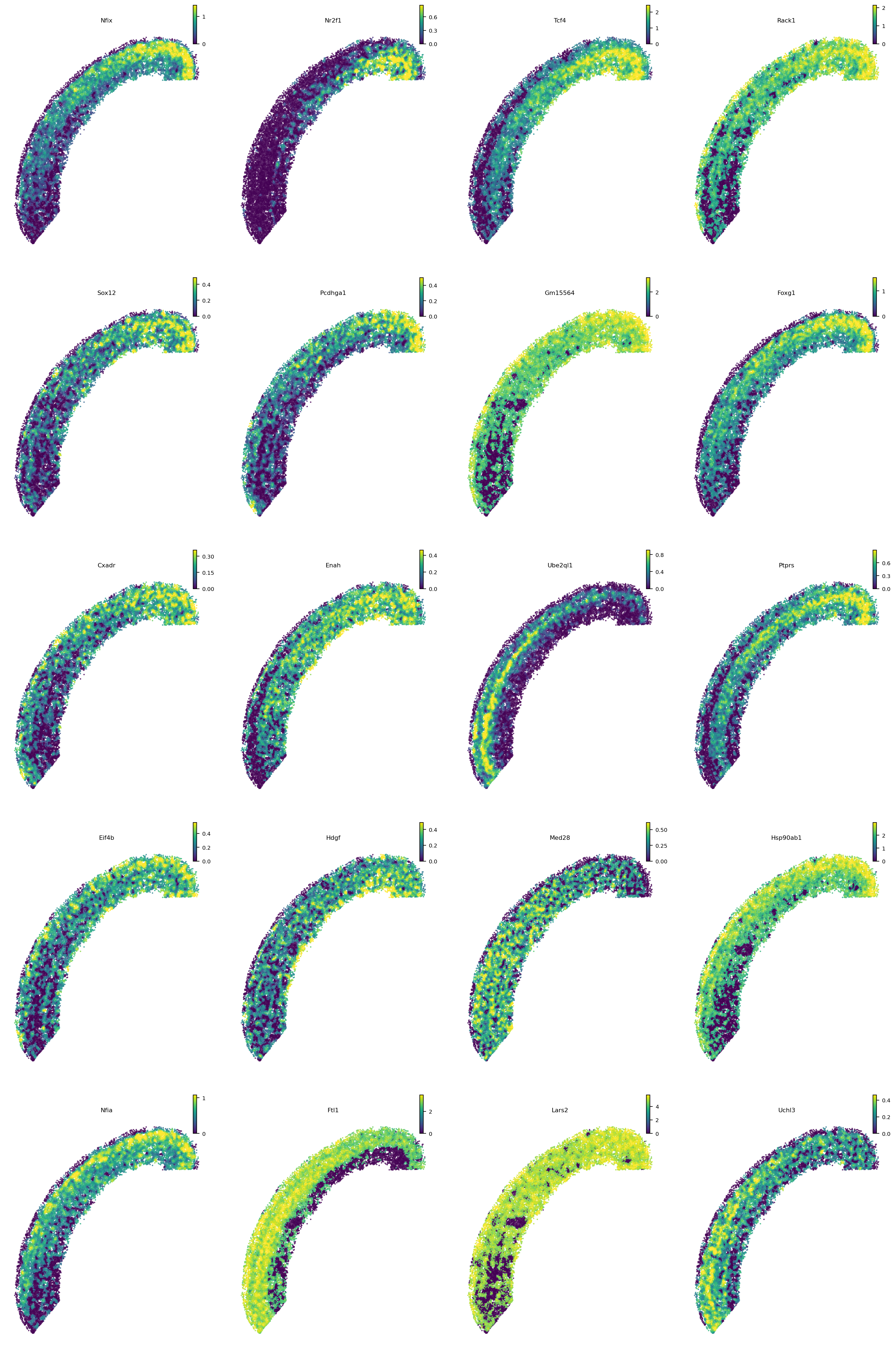
Show top 20 genes#
[7]:
st.pl.space(e16_sm, color=sig_df.sort_values(by='log2fc', ascending=False).index[0:20], pointsize=0.1, show_legend="upper left", space='spatial')
Identify genes have similar spatial expression patterns to specific genes#
[8]:
e16_gene_w, _ = st.svg.cal_wass_dis_target_on_genes(e16, n_neighbors=8, target_genes=["Neurod1", 'Fabp7'], processes=7, bootstrap=100, min_dis_cutoff=500, max_dis_cutoff=1000,)
|-----> Start computing neighbor graph...
|-----> method arg is None, choosing methods automatically...
|-----------> method kd_tree selected
|-----> <insert> spatial_connectivities to obsp in AnnData Object.
|-----> <insert> spatial_distances to obsp in AnnData Object.
|-----> <insert> spatial_neighbors to uns in AnnData Object.
|-----> <insert> spatial_neighbors.indices to uns in AnnData Object.
|-----> <insert> spatial_neighbors.params to uns in AnnData Object.
|-----> The cell/buckets number after filtering by min_dis_cutoff is 400
|-----> The cell/buckets number after filtering by max_dis_cutoff is 400
|-----> Start computing neighbor graph...
|-----> method arg is None, choosing methods automatically...
|-----------> method kd_tree selected
|-----> <insert> spatial_connectivities to obsp in AnnData Object.
|-----> <insert> spatial_distances to obsp in AnnData Object.
|-----> <insert> spatial_neighbors to uns in AnnData Object.
|-----> <insert> spatial_neighbors.indices to uns in AnnData Object.
|-----> <insert> spatial_neighbors.params to uns in AnnData Object.
|-----> The cell/buckets number after filtering by min_dis_cutoff is 400
|-----> The cell/buckets number after filtering by max_dis_cutoff is 400
|-----> Start computing neighbor graph...
|-----> method arg is None, choosing methods automatically...
|-----------> method kd_tree selected
|-----> <insert> spatial_connectivities to obsp in AnnData Object.
|-----> <insert> spatial_distances to obsp in AnnData Object.
|-----> <insert> spatial_neighbors to uns in AnnData Object.
|-----> <insert> spatial_neighbors.indices to uns in AnnData Object.
|-----> <insert> spatial_neighbors.params to uns in AnnData Object.
100%|██████████| 100/100 [00:07<00:00, 14.00it/s]
|-----> Start computing neighbor graph...
|-----> method arg is None, choosing methods automatically...
|-----------> method kd_tree selected
|-----> <insert> spatial_connectivities to obsp in AnnData Object.
|-----> <insert> spatial_distances to obsp in AnnData Object.
|-----> <insert> spatial_neighbors to uns in AnnData Object.
|-----> <insert> spatial_neighbors.indices to uns in AnnData Object.
|-----> <insert> spatial_neighbors.params to uns in AnnData Object.
|-----> The cell/buckets number after filtering by min_dis_cutoff is 400
|-----> The cell/buckets number after filtering by max_dis_cutoff is 400
|-----> Start computing neighbor graph...
|-----> method arg is None, choosing methods automatically...
|-----------> method kd_tree selected
|-----> <insert> spatial_connectivities to obsp in AnnData Object.
|-----> <insert> spatial_distances to obsp in AnnData Object.
|-----> <insert> spatial_neighbors to uns in AnnData Object.
|-----> <insert> spatial_neighbors.indices to uns in AnnData Object.
|-----> <insert> spatial_neighbors.params to uns in AnnData Object.
100%|██████████| 100/100 [00:12<00:00, 7.70it/s]
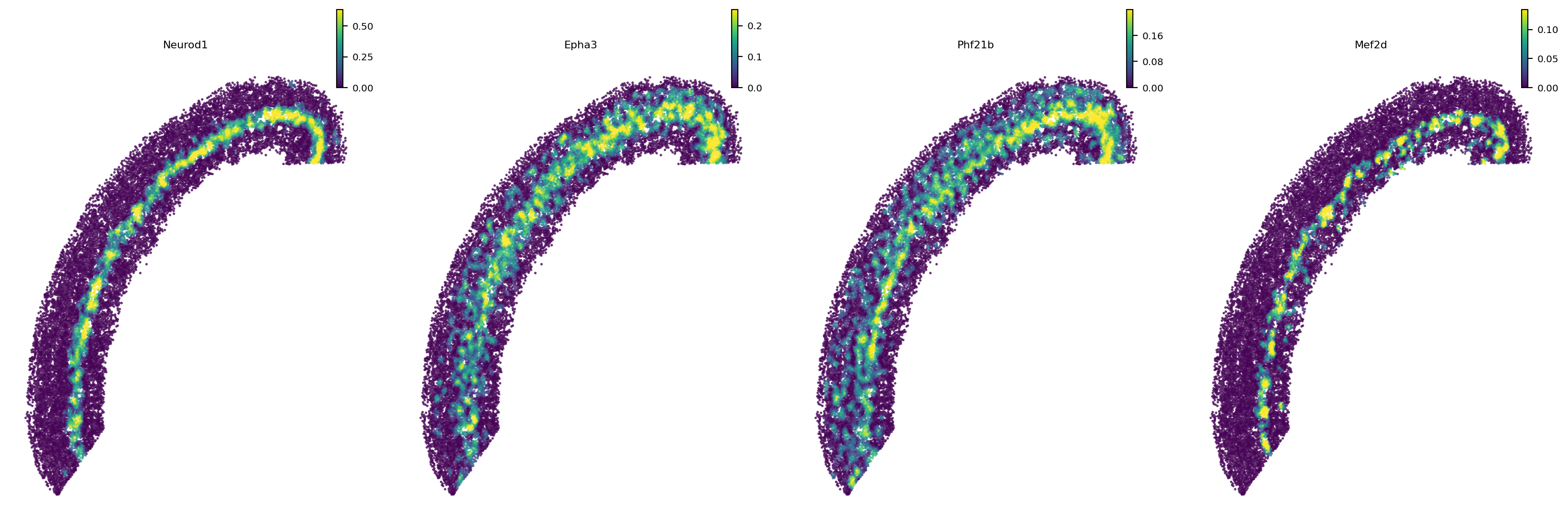
[9]:
# Top 10 genes are similar to Neurod1
e16_gene_w['Neurod1'].sort_values(by='Wasserstein_distance').head(10)
[9]:
| Wasserstein_distance | positive_ratio | mean | std | zscore | pvalue | adj_pvalue | fc | log2fc | -log10adjp | |
|---|---|---|---|---|---|---|---|---|---|---|
| gene_id | ||||||||||
| Neurod1 | 0.000000 | 0.2400 | 426.566569 | 110.729600 | -3.852326 | 0.000059 | 0.005077 | 0.000000 | -inf | 2.294414 |
| Epha3 | 109.124797 | 0.5200 | 407.132366 | 80.676812 | -3.693844 | 0.000110 | 0.008688 | 0.268033 | -1.899519 | 2.061098 |
| Phf21b | 114.516812 | 0.5675 | 404.575468 | 84.986447 | -3.412999 | 0.000321 | 0.019514 | 0.283054 | -1.820849 | 1.709653 |
| Mef2d | 122.587974 | 0.1975 | 459.033970 | 158.322466 | -2.125068 | 0.016790 | 0.072109 | 0.267056 | -1.904783 | 1.142008 |
| Ccdc88c | 144.452329 | 0.7150 | 393.574910 | 59.047196 | -4.219042 | 0.000012 | 0.001214 | 0.367026 | -1.446045 | 2.915882 |
| 2510009E07Rik | 146.244516 | 0.3150 | 434.941081 | 102.262324 | -2.823098 | 0.002378 | 0.046562 | 0.336240 | -1.572437 | 1.331973 |
| 2700081O15Rik | 152.519340 | 0.7075 | 404.019346 | 65.160622 | -3.859693 | 0.000057 | 0.004983 | 0.377505 | -1.405432 | 2.302511 |
| D630045J12Rik | 153.715651 | 0.2525 | 443.881697 | 127.091730 | -2.283123 | 0.011212 | 0.072109 | 0.346299 | -1.529911 | 1.142008 |
| Mex3a | 154.838818 | 0.7200 | 390.877699 | 53.383862 | -4.421540 | 0.000005 | 0.000495 | 0.396131 | -1.335950 | 3.305589 |
| Trp53inp2 | 158.934451 | 0.7250 | 402.398483 | 57.723664 | -4.217751 | 0.000012 | 0.001214 | 0.394968 | -1.340193 | 2.915882 |
[10]:
# Show example genes
st.pl.space(e16_sm, color=['Neurod1', 'Epha3', 'Phf21b', 'Mef2d'], pointsize=0.1, show_legend="upper left", space='spatial')
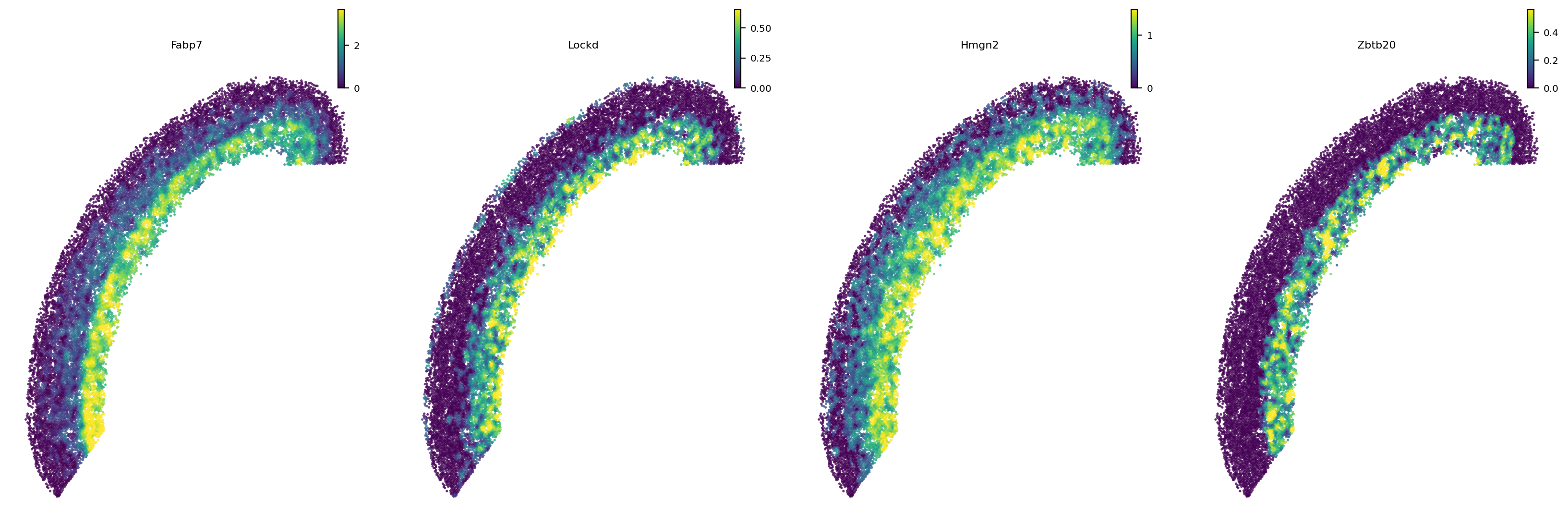
[11]:
# Top 10 genes are similar to Fabp7
e16_gene_w['Fabp7'].sort_values(by='Wasserstein_distance').head(10)
[11]:
| Wasserstein_distance | positive_ratio | mean | std | zscore | pvalue | adj_pvalue | fc | log2fc | -log10adjp | |
|---|---|---|---|---|---|---|---|---|---|---|
| gene_id | ||||||||||
| Fabp7 | 0.000000 | 0.7125 | 382.119183 | 80.226183 | -4.763023 | 9.535687e-07 | 0.000093 | 0.000000 | -inf | 4.029442 |
| Lockd | 53.788738 | 0.5100 | 381.800645 | 82.260702 | -3.987468 | 3.339112e-05 | 0.002568 | 0.140882 | -2.827444 | 2.590429 |
| Hmgn2 | 59.864920 | 0.7050 | 374.260007 | 60.587304 | -5.189125 | 1.056423e-07 | 0.000011 | 0.159955 | -2.644258 | 4.976164 |
| Ccdc115 | 61.983720 | 0.5025 | 386.175798 | 85.063690 | -3.811169 | 6.915565e-05 | 0.004761 | 0.160506 | -2.639297 | 2.322344 |
| Nmt1 | 67.239757 | 0.3550 | 395.432131 | 90.707347 | -3.618145 | 1.483608e-04 | 0.008274 | 0.170041 | -2.556044 | 2.082264 |
| H2afz | 70.602171 | 0.7025 | 374.652324 | 65.553335 | -4.638210 | 1.757196e-06 | 0.000169 | 0.188447 | -2.407768 | 3.772945 |
| Zbtb20 | 71.213793 | 0.4050 | 391.138576 | 92.670357 | -3.452288 | 2.779268e-04 | 0.013528 | 0.182068 | -2.457451 | 1.868767 |
| Pea15a | 73.291279 | 0.7150 | 375.614612 | 67.891255 | -4.453053 | 4.232900e-06 | 0.000394 | 0.195124 | -2.357540 | 3.404964 |
| H2afv | 76.786626 | 0.7125 | 368.835558 | 54.667684 | -5.342259 | 4.589767e-08 | 0.000005 | 0.208187 | -2.264051 | 5.333889 |
| Cdk4 | 78.616330 | 0.5425 | 373.354204 | 70.350766 | -4.189547 | 1.397557e-05 | 0.001173 | 0.210568 | -2.247644 | 2.930603 |
[12]:
# Show example genes
st.pl.space(e16_sm, color=['Fabp7', 'Lockd', 'Hmgn2', 'Zbtb20'], pointsize=0.1, show_legend="upper left", space='spatial')
[ ]: