Note

This page was generated from 3_ligand_receptor_specfic_enrichment_analysis.ipynb. Interactive online version: . Some tutorial content may look better in light mode.

Ligand receptor specfic enrichment analysis.

This notebook demonstrates ligand-specific enrichment analysis. Similar to the differential gene analysis, We can observe that the ligand receptor pair specifically enriched in a certain spatial region. This is done in the following three steps.

1. Construct a new anndata object, in which the columns of the matrix are cell-cell pairs, while the rows ligand-receptor mechanisms.

2. Based on above matrix, do dimensionality reduction,spatial clustering and differential mechanisms (ligand-receptor) analysis, to find the specifically enriched in a certain spatial region.

Reference: Micha Sam Brickman Raredon, Junchen Yang, Neeharika Kothapalli, Naftali Kaminski, Laura E. Niklason,Yuval Kluger. Comprehensive visualization of cell-cell interactions in single-cell and spatial transcriptomics with NICHES. doi: https://doi.org/10.1101/2022.01.23.477401

import os
import spateo as st
import dynamo as dyn
import matplotlib.pyplot as plt
import seaborn as sns
import pandas as pd
import numpy as np

Load data

We will be using a axolotl dataset from [Wei et al., 2022] (https://doi.org/10.1126/science.abp9444).

Here, we can get data directly from the functionst.sample.axolotl or link:

axolotl_2DPI: https://www.dropbox.com/s/7w2jxf41xazrqxo/axolotl_2DPI.h5ad?dl=1

adata = st.sample_data.axolotl(filename='axolotl_2DPI.h5ad')
adata

AnnData object with n_obs × n_vars = 7668 × 27324
    obs: 'CellID', 'spatial_leiden_e30_s8', 'Batch', 'cell_id', 'seurat_clusters', 'inj_uninj', 'D_V', 'inj_M_L', 'Annotation'
    var: 'Axolotl_ID', 'hs_gene'
    uns: 'Annotation_colors', '__type', 'color_key'
    obsm: 'X_spatial', 'spatial'
    layers: 'counts', 'log1p'
    obsp: 'connectivities', 'distances', 'spatial_connectivities', 'spatial_distances'

adata.var['new_name'] = adata.var.index
adata.var.index = adata.var['Axolotl_ID']

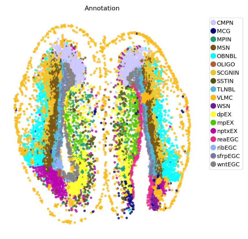
st.pl.space(adata,
            color=['Annotation'],
            pointsize=0.2,
            color_key=adata.uns['color_key'],
            show_legend='upper left',
            figsize=(5, 5))

Construct new adata.

First, calculate spatial nearest neighbor graph, limiting the nearest neighbor per cell to k. This function returns another anndata object, in which the columns of the matrix are cell-cell pairs, while the rows ligand-receptor mechanisms.

weights_graph, distance_graph, adata = st.tl.weighted_spatial_graph(
    adata,
    n_neighbors=10,
)

|-----> <insert> spatial_connectivities to obsp in AnnData Object.
|-----> <insert> spatial_distances to obsp in AnnData Object.
|-----> <insert> spatial_neighbors to uns in AnnData Object.
|-----> <insert> spatial_neighbors.indices to uns in AnnData Object.
|-----> <insert> spatial_neighbors.params to uns in AnnData Object.
|-----> <insert> spatial_weights to obsp in AnnData Object.

adata_n2n = st.tl.niches(adata,
                         path='/DATA/User/zuolulu/spateo-release/spateo/tools/database/',
                         layer=None,
                         species='axolotl',
                         system='niches_n2n',
                         method='sum')
adata_n2n

AnnData object with n_obs × n_vars = 7668 × 916
    obs: 'cell_pair_name'

Copy some of the other attributes from adata to adata_n2n. (Note assignment based on actual data).

adata_n2n.uns['__type'] = 'UMI'
adata_n2n.obsm['spatial'] = adata.obsm['spatial']

Downstream analysis.

Then, we can do dimensionality reduction , spatial clustering and differential mechanisms (ligand-receptor) analysis based on this new object. Therefore, we can find the ligand-receptor pairs which are specially enriched in a certain region.

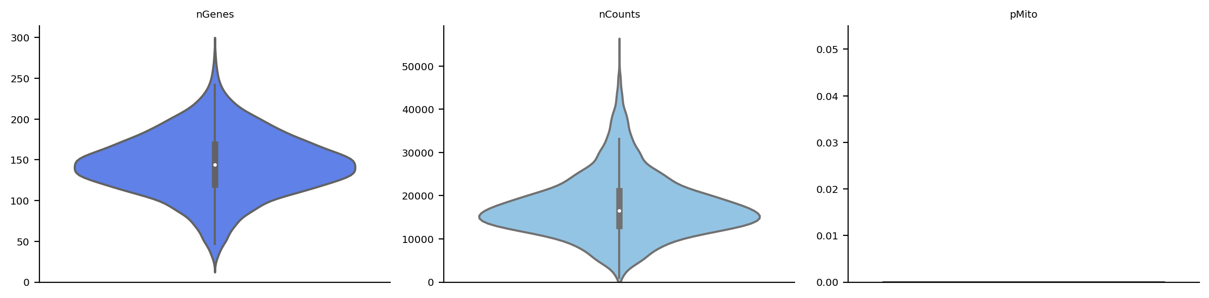
preprocessing

adata_n2n.obs['n_counts'] = adata_n2n.X.sum(axis=1).A1
adata_n2n.uns["pp"] = {}
adata_n2n.var_names_make_unique()
dyn.pl.basic_stats(adata_n2n)
adata_n2n.layers['raw'] = adata_n2n.X
dyn.pp.normalize_cell_expr_by_size_factors(adata_n2n, layers="X")
adata_n2n.layers['norm_log1p'] = adata_n2n.X.copy()
adata_n2n.X = adata_n2n.layers['raw'].copy()
st.tl.pearson_residuals(adata_n2n, n_top_genes=None)
adata_n2n

|-----> rounding expression data of layer: X during size factor calculation
|-----> size factor normalize following layers: ['X']
|-----> applying <ufunc 'log1p'> to layer<X>
|-----> set adata <X> to normalized data.
|-----> <insert> pp.norm_method to uns in AnnData Object.

AnnData object with n_obs × n_vars = 7668 × 916
    obs: 'cell_pair_name', 'n_counts', 'nGenes', 'nCounts', 'pMito', 'Size_Factor', 'initial_cell_size'
    var: 'nCells', 'nCounts'
    uns: '__type', 'pp'
    obsm: 'spatial', 'pearson_residuals'
    layers: 'raw', 'norm_log1p'

bad_genes = np.isnan(adata_n2n.obsm["pearson_residuals"].sum(0))
bad_genes.sum()
st.tl.pca_spateo(adata=adata_n2n, X_data=adata_n2n.obsm["pearson_residuals"]
                 [:, ~bad_genes], n_pca_components=30, pca_key="X_pca", random_state=1)
dyn.tl.neighbors(adata_n2n, n_neighbors=30)

|-----> Runing PCA on user provided data...
|-----> Start computing neighbor graph...
|-----------> X_data is None, fetching or recomputing...
|-----> fetching X data from layer:None, basis:pca
|-----> method arg is None, choosing methods automatically...
|-----------> method ball_tree selected
|-----> <insert> connectivities to obsp in AnnData Object.
|-----> <insert> distances to obsp in AnnData Object.
|-----> <insert> neighbors to uns in AnnData Object.
|-----> <insert> neighbors.indices to uns in AnnData Object.
|-----> <insert> neighbors.params to uns in AnnData Object.

AnnData object with n_obs × n_vars = 7668 × 916
    obs: 'cell_pair_name', 'n_counts', 'nGenes', 'nCounts', 'pMito', 'Size_Factor', 'initial_cell_size'
    var: 'nCells', 'nCounts'
    uns: '__type', 'pp', 'neighbors'
    obsm: 'spatial', 'pearson_residuals', 'X_pca'
    layers: 'raw', 'norm_log1p'
    obsp: 'distances', 'connectivities'

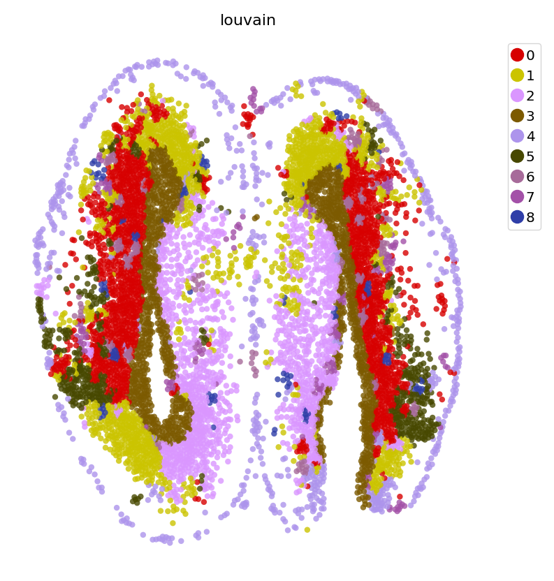
clustering

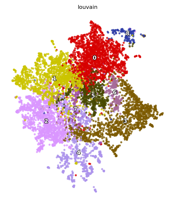
dyn.tl.louvain(adata_n2n, resolution=2)
st.pl.space(adata_n2n,
            color=['louvain'],
            pointsize=0.2,
            figsize=(5, 5),
            show_legend="upper left")
dyn.tl.reduceDimension(adata_n2n)
st.pl.space(adata_n2n,
            color=['louvain'],
            figsize=(5, 5),
            space="umap",
            pointsize=0.2)

|-----> accessing adj_matrix_key=distances built from args for clustering...
|-----> Detecting communities on graph...
|-----------> Converting graph_sparse_matrix to networkx object
|-----> [Community clustering with louvain] in progress: 100.0000%
|-----> [Community clustering with louvain] finished [412.6376s]

|-----> retrive data for non-linear dimension reduction...
|-----> perform umap...
|-----> [dimension_reduction projection] in progress: 100.0000%
|-----> [dimension_reduction projection] finished [43.6265s]

differential analysis

# (optional: just Suitable for axolotl, homologous gene to human)
#adata_n2n.var['lr_pair_name'] = adata_n2n.var.index
df = adata_n2n.var['lr_pair_name'].str.split('-', expand=True)
df.columns = ['ligand', 'receptor']
##
df1 = adata.var
df1.index.name = None
df2 = pd.merge(df, df1, left_on='ligand', right_on='Axolotl_ID').drop(
    ['Axolotl_ID', 'new_name'], axis=1)
df2.columns = ['ligand', 'receptor', 'ligand_human']
df3 = pd.merge(df2, df1, left_on='receptor',
               right_on='Axolotl_ID').drop(['Axolotl_ID', 'new_name'], axis=1)
df3.columns = ['ligand', 'receptor', 'ligand_human', 'receptor_human']
df3['ligand_human'] = df3['ligand_human'].astype('str')
df3['receptor_human'] = df3['receptor_human'].astype('str')
df3['lr_pair'] = df3["ligand_human"] + "-" + df3["receptor_human"]
adata_n2n.var['lr_pair'] = df3['lr_pair'].tolist()
adata_n2n.var.index = adata_n2n.var['lr_pair']

adata_n2c_marker = st.tl.find_all_cluster_degs(
    adata_n2n, group='louvain', genes=None, n_jobs=1)

identifying top markers for each group: 916it [00:04, 223.56it/s]
identifying top markers for each group: 916it [00:04, 214.35it/s]
identifying top markers for each group: 916it [00:04, 199.74it/s]
identifying top markers for each group: 916it [00:05, 178.17it/s]
identifying top markers for each group: 916it [00:04, 224.85it/s]
identifying top markers for each group: 916it [00:03, 236.41it/s]
identifying top markers for each group: 916it [00:04, 217.55it/s]
identifying top markers for each group: 916it [00:04, 201.59it/s]
identifying top markers for each group: 916it [00:04, 204.19it/s]

# top_n_markers
marker_genes_dict = st.tl.top_n_degs(
    adata_n2c_marker, group='louvain', top_n_genes=3)

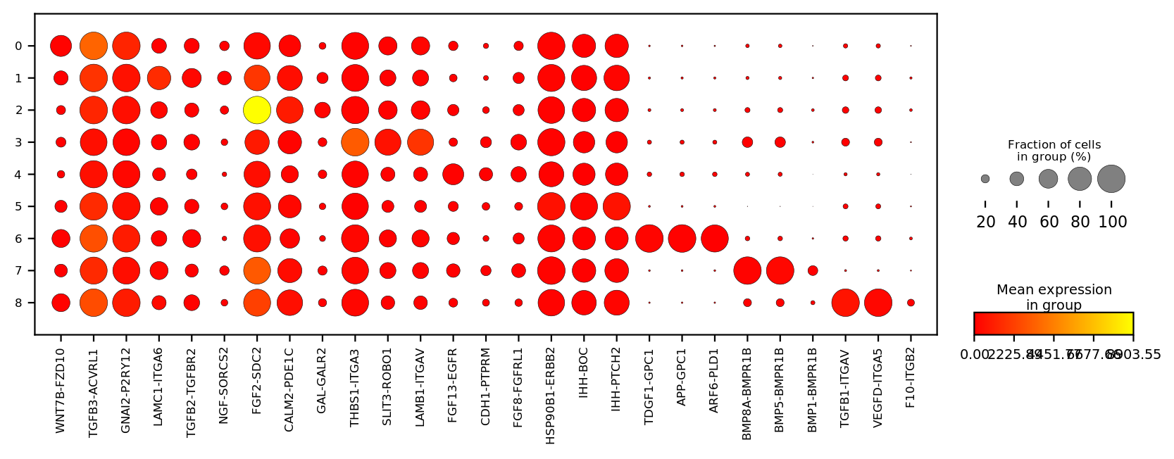
deg_table = st.tl.top_n_degs(adata_n2c_marker, group='louvain',
                             only_deg_list=False, sort_by='cosine_score', top_n_genes=3)

markers = deg_table['gene'].unique().tolist()
adata_n2n.var_names_make_unique()
adata_n2n.obs['louvain'] = adata_n2n.obs['louvain'].astype('category')

st.pl.dotplot(adata_n2n,
              var_names=markers,
              cat_key='louvain',
              cmap='autumn',
              figsize=(10, 3),
              save_show_or_return='return')

(<Figure size 1000x300 with 4 Axes>,
 {'mainplot_ax': <AxesSubplot:>,
  'size_legend_ax': <AxesSubplot:title={'center':'Fraction of cells\nin group (%)'}>,
  'color_legend_ax': <AxesSubplot:title={'center':'Mean expression\nin group'}>})

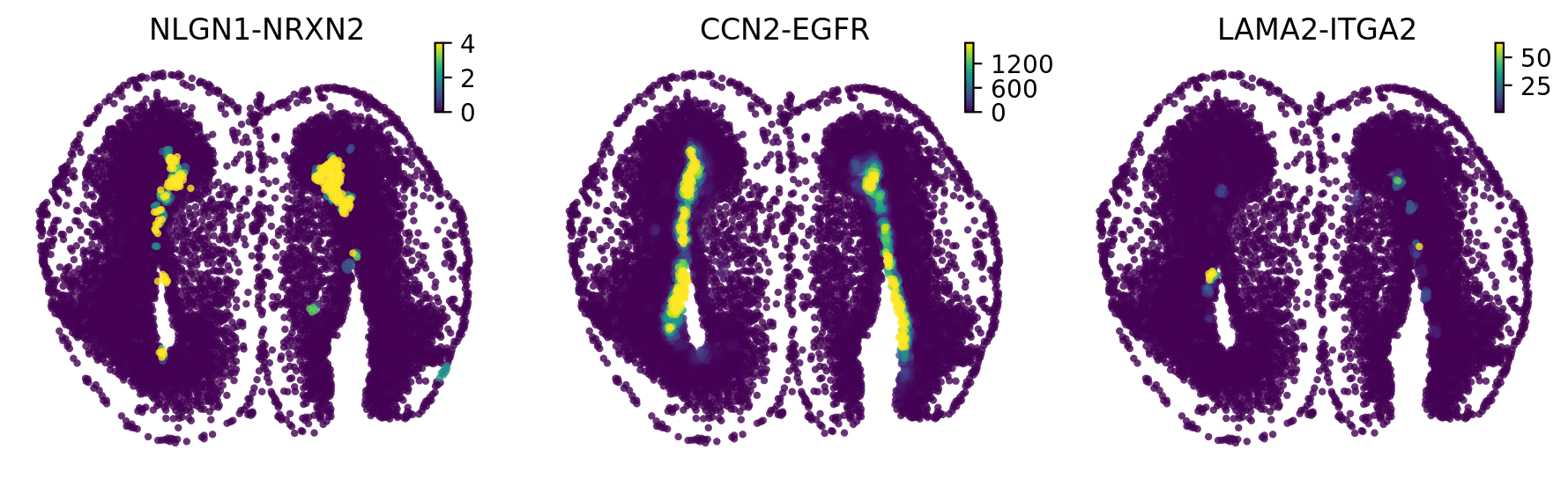
Plot spatial in situ expression map

st.pl.space(adata_n2n,
            color=marker_genes_dict['3'],
            pointsize=0.2,
            ncols=3,
            figsize=(4, 3),
            show_legend="upper left")