Note

This page was generated from 4_svg_archetype.ipynb. Interactive online version: . Some tutorial content may look better in light mode.

4.Identification of spatial variable genes and archetypes

This notebook demonstrates how to use spateo to identify spatial variable genes, by calculating Moran‘s I score, and how to get spatial gene archetypes.

import spateo as st

import numpy as np

st.configuration.set_pub_style_mpltex()
%matplotlib inline

2022-11-13 20:18:33.040154: I tensorflow/core/util/util.cc:169] oneDNN custom operations are on. You may see slightly different numerical results due to floating-point round-off errors from different computation orders. To turn them off, set the environment variable `TF_ENABLE_ONEDNN_OPTS=0`.
network.py (36): The next major release of pysal/spaghetti (2.0.0) will drop support for all ``libpysal.cg`` geometries. This change is a first step in refactoring ``spaghetti`` that is expected to result in dramatically reduced runtimes for network instantiation and operations. Users currently requiring network and point pattern input as ``libpysal.cg`` geometries should prepare for this simply by converting to ``shapely`` geometries.

Data source

bin60_clustered_h5ad: https://www.dropbox.com/s/wxgkim87uhpaz1c/mousebrain_bin60_clustered.h5ad?dl=0

# Load annotated binning data
fname_bin60 = "mousebrain_bin60_clustered.h5ad"
adata_bin60 = st.sample_data.mousebrain(fname_bin60)

adata_bin60

AnnData object with n_obs × n_vars = 7765 × 21667
    obs: 'area', 'n_counts', 'Size_Factor', 'initial_cell_size', 'louvain', 'scc', 'scc_anno'
    var: 'pass_basic_filter'
    uns: '__type', 'louvain', 'louvain_colors', 'neighbors', 'pp', 'scc', 'scc_anno_colors', 'scc_colors', 'spatial', 'spatial_neighbors'
    obsm: 'X_pca', 'X_spatial', 'bbox', 'contour', 'spatial'
    layers: 'count', 'spliced', 'unspliced'
    obsp: 'connectivities', 'distances', 'spatial_connectivities', 'spatial_distances'

SVG identification (Moran’s I)

# Filter out low expressed and uninterested, such as mitochondrial genes
mito_genes = adata_bin60.var_names.str.startswith("mt-")
adata_bin60 = adata_bin60[: ,~mito_genes]

st.pp.filter.filter_genes(adata_bin60,min_cells= adata_bin60.n_obs*0.05, inplace=True)
adata_bin60

AnnData object with n_obs × n_vars = 7765 × 5059
    obs: 'area', 'n_counts', 'Size_Factor', 'initial_cell_size', 'louvain', 'scc', 'scc_anno'
    var: 'pass_basic_filter'
    uns: '__type', 'louvain', 'louvain_colors', 'neighbors', 'pp', 'scc', 'scc_anno_colors', 'scc_colors', 'spatial', 'spatial_neighbors'
    obsm: 'X_pca', 'X_spatial', 'bbox', 'contour', 'spatial'
    layers: 'count', 'spliced', 'unspliced'
    obsp: 'connectivities', 'distances', 'spatial_connectivities', 'spatial_distances'

# Calculate Moran's I score for genes
m = st.tl.moran_i(adata_bin60, n_jobs=30)

# Filter genes by Moran's I score and adjusted p-value
m_filter = m[(m.moran_i > 0.15)&(m.moran_q_val<0.05)].sort_values(by=['moran_i'],ascending=False)
m_filter[0:10]

	moran_i	moran_p_val	moran_z	moran_q_val
Plp1	0.529320	0.005	78.720267	0.014116
Gm28928	0.516217	0.005	72.395455	0.014116
Ntng1	0.511843	0.005	72.667184	0.014116
Mbp	0.510432	0.005	77.079408	0.014116
Gm42418	0.468743	0.005	69.624860	0.014116
Phactr1	0.468161	0.005	70.079342	0.014116
Mobp	0.457718	0.005	61.732588	0.014116
Cmss1	0.436734	0.005	65.651464	0.014116
Kcnip4	0.421696	0.005	61.525662	0.014116
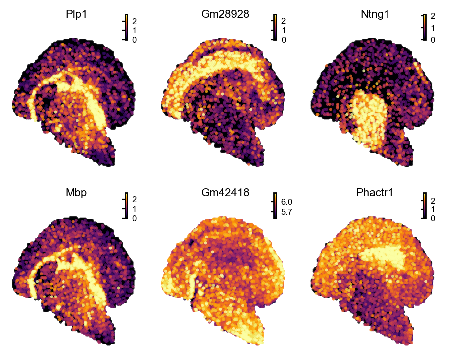
Camk1d	0.406778	0.005	56.055133	0.014116

# Visualize top SVGs
st.pl.space(
    adata_bin60,
    genes=m_filter.index[0:6].tolist(),
    pointsize=0.1,
    ncols=3,
    show_legend="upper left",
    figsize=(2,2),
)

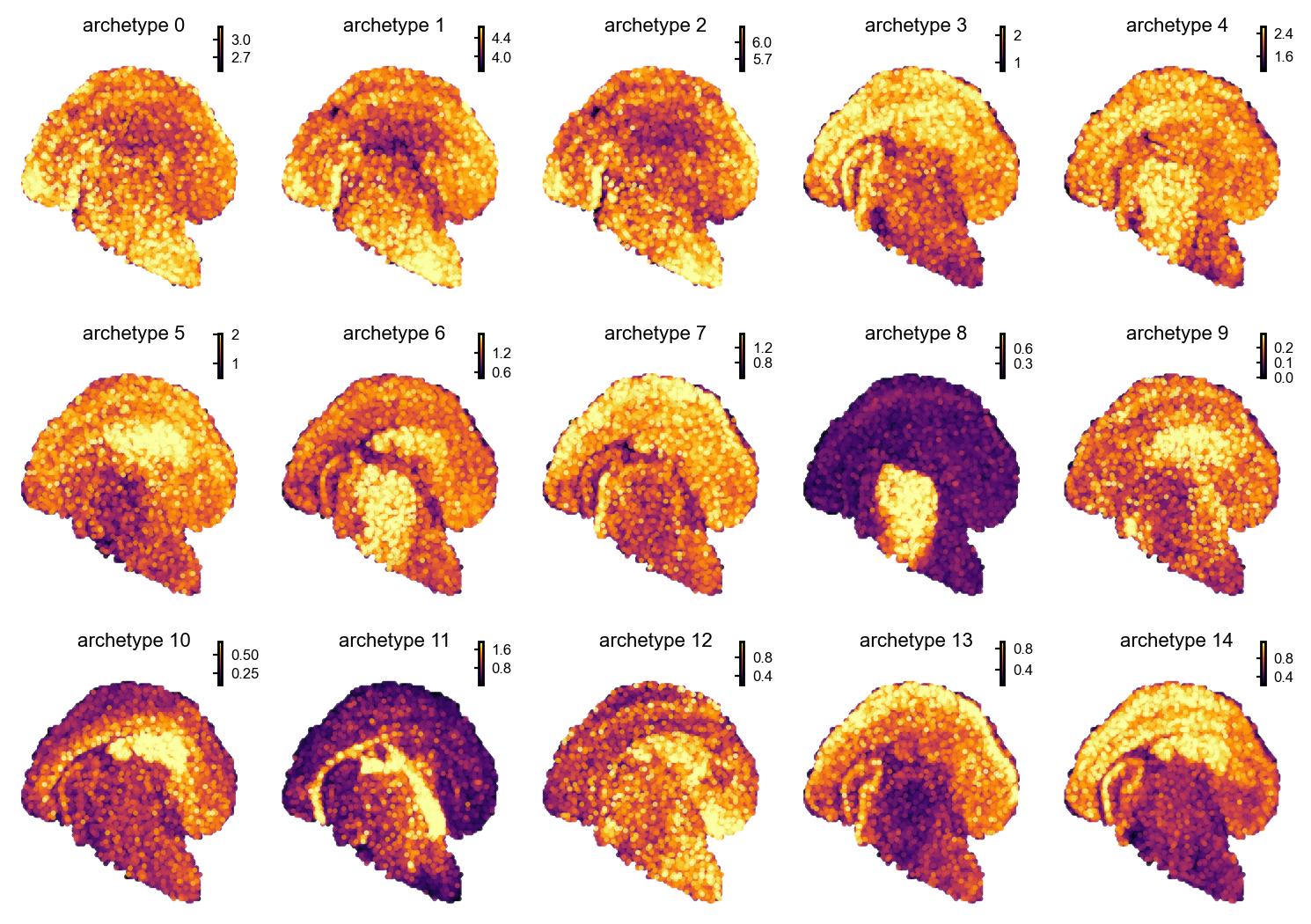
SVG archetypes

# Cluster identified SVGs into archetypes
num_clusters = 15

archetypes, clusters, gene_corrs = st.tl.find_spatial_archetypes(
    exp_mat = adata_bin60[:,m_filter.index].X.A.T,
    num_clusters = num_clusters,
)

|-----> [Finding gene archetypes] in progress: 100.0000%
|-----> [Finding gene archetypes] finished [0.1889s]
|-----> done!

# Create dataframe with genes and its archetype
df_clusters = pd.DataFrame({"gene":m_filter.index.to_list(), "archetype":clusters-1})
df_clusters[0:10]

# Save gene cluster info
# df_clusters.to_csv("archetype_clusters.csv")

	gene	archetype
0	Plp1	11
1	Gm28928	14
2	Ntng1	8
3	Mbp	11
4	Gm42418	2
5	Phactr1	5
6	Mobp	11
7	Cmss1	1
8	Kcnip4	4
9	Camk1d	1

# Calculate genes having significant spatial correlation with each archetype
archetypes_dict = st.tl.archetypes_genes(
    adata=adata_bin60,
    archetypes=archetypes,
    num_clusters=num_clusters,
    moran_i_genes=m_filter.index,
)

|-----? No genes with significant correlation were found at the current p-value threshold.

# Calculate expression scores for archetypes
adata_bin60.obs = st.tl.archetypes(adata_bin60,m_filter.index,num_clusters=num_clusters)

|-----> [Finding gene archetypes] in progress: 100.0000%
|-----> [Finding gene archetypes] finished [0.1891s]
|-----> done!

# Visualize archetypes
arch_cols = ["archetype %d" % i for i in np.arange(num_clusters)]
st.pl.space(
    adata_bin60,
    color = adata_bin60.obs[arch_cols].columns.tolist(),
    pointsize=0.1,
    ncols=5,
    show_legend="upper left",
    figsize=(2,2),
)