Note
This page was generated from
1_cell-cell_communication_inference.ipynb.
Interactive online version:
![]() .
Some tutorial content may look better in light mode.
.
Some tutorial content may look better in light mode.
cell-cell communication inference#
In this tutorial, we demonstrate the cell cell interaction based on ligand-receptor products conditioned on spatial proximity between clusters. This is done in the following three steps.
Find spatially adjacent clusters(celltypes);
Given two celltypes, find space-specific ligand-receptor pairs.
(Optional),Loop executes multiple two-cell type interactions.
[ ]:
import numpy as np
import pandas as pd
import seaborn as sns
import matplotlib.pyplot as plt
import spateo as st
Load data#
We will be using a axolotl dataset from [Wei et al., 2022] (https://doi.org/10.1126/science.abp9444).
Here, we can get data directly from the functionst.sample.axolotl or link:
axolotl_2DPI: https://www.dropbox.com/s/7w2jxf41xazrqxo/axolotl_2DPI.h5ad?dl=1
axolotl_2DPI_right: https://www.dropbox.com/s/pm5vvqcd4leahsb/axolotl_2DPI_right.h5ad?dl=1
[2]:
adata = st.sample_data.axolotl(filename='axolotl_2DPI.h5ad')
adata
[2]:
AnnData object with n_obs × n_vars = 7668 × 27324
    obs: 'CellID', 'spatial_leiden_e30_s8', 'Batch', 'cell_id', 'seurat_clusters', 'inj_uninj', 'D_V', 'inj_M_L', 'Annotation'
    var: 'Axolotl_ID', 'hs_gene'
    uns: 'Annotation_colors', '__type', 'color_key'
    obsm: 'X_spatial', 'spatial'
    layers: 'counts', 'log1p'
    obsp: 'connectivities', 'distances', 'spatial_connectivities', 'spatial_distances'
[3]:
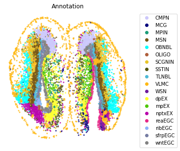
st.pl.space(adata,
            color=['Annotation'],
            pointsize=0.2,
            color_key=adata.uns['color_key'],
            show_legend='upper left',
            figsize=(5, 5))
Find spatially adjacent celltypes#
First, we calculate the weighted spatial graph between celltypes, which the nearest neighbor of a cell are based on the fixed-neighbor or fixed-radius methods. The spatial graphs and spatial distances are saves to adata.obsp['spatial_distances'],adata.obsp['spatial_weights'],adata.obsp['spatial_connectivities'] ,adata.uns['spatial_neighbors'].
[4]:
weights_graph, distance_graph, adata = st.tl.weighted_spatial_graph(
    adata,
    n_neighbors=10,
    fixed='n_neighbors',
)
|-----> <insert> spatial_connectivities to obsp in AnnData Object.
|-----> <insert> spatial_distances to obsp in AnnData Object.
|-----> <insert> spatial_neighbors to uns in AnnData Object.
|-----> <insert> spatial_neighbors.indices to uns in AnnData Object.
|-----> <insert> spatial_neighbors.params to uns in AnnData Object.
|-----> <insert> spatial_weights to obsp in AnnData Object.
[5]:
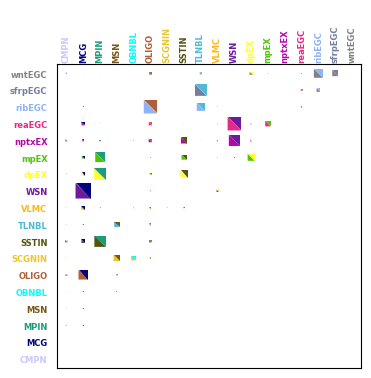
st.pl.plot_connections(
    adata,
    cat_key='Annotation',
    save_show_or_return='show',
    title_str=" ",
    title_fontsize=6,
    label_fontsize=6,
    colormap=adata.uns['color_key'],
    figsize=(4, 4),
)
|-----> <insert> spatial_connectivities to obsp in AnnData Object.
|-----> <insert> spatial_distances to obsp in AnnData Object.
|-----> <insert> spatial_neighbors to uns in AnnData Object.
|-----> <insert> spatial_neighbors.indices to uns in AnnData Object.
|-----> <insert> spatial_neighbors.params to uns in AnnData Object.
|-----> <insert> spatial_weights to obsp in AnnData Object.
|----->
--- 18 labels, 7668 samples ---
initalized (19,) index ptr: [0 0 0 0 0 0 0 0 0 0 0 0 0 0 0 0 0 0 0]
initalized (7668,) indices: [0 0 0 ... 0 0 0]
initalized (7668,) data: [1 1 1 ... 1 1 1]

|-----> Deep copying AnnData object and working on the new copy. Original AnnData object will not be modified.
|-----> Matrix multiplying labels x weights x labels-transpose, shape (18, 7668) x (7668, 7668) x (7668, 18).
Given two celltypes, find space-specific ligand-receptor pairs.#
Based on the result above, here we take the reaEGC(sender celltype) and WSN(receiver celltype) as an example.
[ ]:
adata = st.sample_data.axolotl(filename='axolotl_2DPI_right.h5ad')
adata
AnnData object with n_obs × n_vars = 3625 × 27324
    obs: 'CellID', 'spatial_leiden_e30_s8', 'Batch', 'cell_id', 'seurat_clusters', 'inj_uninj', 'D_V', 'inj_M_L', 'Annotation'
    var: 'Axolotl_ID', 'hs_gene'
    uns: 'Annotation_colors', '__type', 'color_key'
    obsm: 'X_pca', 'X_spatial', 'spatial'
    varm: 'PCs'
    layers: 'counts'
    obsp: 'connectivities', 'distances', 'spatial_connectivities', 'spatial_distances'
[7]:
sender_ct = 'reaEGC'
receptor_ct = 'WSN'
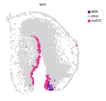
plot all cell pair
[8]:
st.tl.prepare_cci_cellpair_adata(adata, sender_group=sender_ct,
                                 receiver_group=receptor_ct, group='Annotation', all_cell_pair=True)
# plot all cell pair
st.pl.space(adata,
            color=['spec'],
            pointsize=0.2,
            color_key={'other': '#D3D3D3', sender_ct: adata.uns['color_key']
                       [sender_ct], receptor_ct: adata.uns['color_key'][receptor_ct]},
            show_legend='upper left',
            figsize=(4, 4),
            save_show_or_return='show',
            #save_kwargs={"prefix": "./figures/left_2DPI_uninjury_cci_" + sender_ct + "_" + receptor_ct + "_all_cell_pair"}
            )
st.tl.find_cci_two_group
[9]:
weights_graph, distance_graph, adata = st.tl.weighted_spatial_graph(
    adata,
    n_neighbors=10,
)
|-----> <insert> spatial_connectivities to obsp in AnnData Object.
|-----> <insert> spatial_distances to obsp in AnnData Object.
|-----> <insert> spatial_neighbors to uns in AnnData Object.
|-----> <insert> spatial_neighbors.indices to uns in AnnData Object.
|-----> <insert> spatial_neighbors.params to uns in AnnData Object.
|-----> <insert> spatial_weights to obsp in AnnData Object.
[10]:
res = st.tl.find_cci_two_group(adata,
                               path='/DATA/User/zuolulu/spateo-release/spateo/tools/database/',
                               species='axolotl',
                               group='Annotation',
                               sender_group=sender_ct,
                               receiver_group=receptor_ct,
                               filter_lr='outer',
                               min_pairs=0,
                               min_pairs_ratio=0,
                               top=20,)
|-----> 20 ligands for cell type reaEGC with highest fraction of prevalence: ['AMEX60DD008914', 'AMEX60DD001392', 'AMEX60DD049490', 'AMEX60DD051636', 'AMEX60DD041932', 'AMEX60DD008951', 'AMEX60DD028699', 'AMEX60DD034565', 'AMEX60DD049502', 'AMEX60DD001946', 'AMEX60DD013396', 'AMEX60DD055544', 'AMEX60DD003208', 'AMEX60DD014882', 'AMEX60DD005285', 'AMEX60DD043190', 'AMEX60DD040292', 'AMEX60DD012285', 'AMEX60DD001694', 'AMEX60DD017034']. Testing interactions involving these genes.
|-----> 20 receptors for cell type WSN with highest fraction of prevalence: ['AMEX60DD000016', 'AMEX60DD055551', 'AMEX60DD049635', 'AMEX60DD018191', 'AMEX60DDU001007023', 'AMEX60DD041858', 'AMEX60DD051542', 'AMEX60DD029326', 'AMEX60DD029929', 'AMEX60DD055467', 'AMEX60DD014152', 'AMEX60DD027855', 'AMEX60DD055776', 'AMEX60DD033101', 'AMEX60DD051881', 'AMEX60DD042067', 'AMEX60DD029894', 'AMEX60DDU001005617', 'AMEX60DD009754', 'AMEX60DD008017']. Testing interactions involving these genes.
100%|██████████| 1000/1000 [00:08<00:00, 124.60it/s]
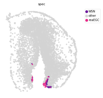
plot spatial neighbors cell pair
[11]:
st.tl.prepare_cci_cellpair_adata(
    adata, sender_group=sender_ct, receiver_group=receptor_ct, cci_dict=res, all_cell_pair=False)
# plot
st.pl.space(adata,
            color=['spec'],
            pointsize=0.2,
            color_key={'other': '#D3D3D3', sender_ct: adata.uns['color_key']
                       [sender_ct], receptor_ct: adata.uns['color_key'][receptor_ct]},
            show_legend='upper left',
            figsize=(4, 4),
            save_show_or_return='return',
            #save_kwargs={"prefix": "./figures/left_2DPI_uninjury_cci_" + sender_ct + "_" + receptor_ct + "_cell_pair"}
            )
[11]:
(None, [<AxesSubplot:title={'center':'spec'}>])
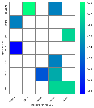
plot heatmap : significant ligand-receptor pairs
From st.tl.find_cci_two_group, we can get significant LR pairs specific to sender and receiver celltypes, res['lr_pair'], with columns are lr_co_exp_num, the number of cell-pairs co-expressed liagnd(expressed in sender cell type) and receptor(expressed in receiver cell type). lr_co_exp_ratio,Co-expressed cell-pairs account for all the paired cells.lr_co_exp_ratio_pvalue,p value of the LR pairs from permutation test, lr_co_exp_ratio_qvalue,FDR value. Here we use heatmap
to show the LR pairs.
[12]:
df = res['lr_pair']
df = df.loc[df['lr_co_exp_num'] > 0].sort_values(
    'lr_co_exp_ratio', ascending=False)[0:10]
[13]:
%matplotlib inline
data1 = df.iloc[:, [2, 3, 7]]
test = data1.pivot(index="human_ligand", columns="human_receptor",
                   values="lr_co_exp_ratio").fillna(0)
fig = plt.figure()
fig.set_size_inches(5, 5)
x_label = list(test.columns.tolist())
y_label = list(test.index)
ax = sns.heatmap(test,
                 cmap="winter",
                 square=True,
                 yticklabels=y_label,
                 linecolor='grey',
                 linewidths=0.3,
                 annot_kws={'size': 10, 'weight': 'bold', },
                 xticklabels=x_label,
                 mask=(test < 0.01))
plt.gcf().subplots_adjust(bottom=0.3)
plt.xlabel("Receptor in reaEGC")
plt.ylabel("Ligand in WSN")
ax.set_xticklabels(x_label, rotation=45, ha="right")
ax.xaxis.set_ticks_position('none')
ax.yaxis.set_ticks_position('none')
plt.tight_layout()
#plt.savefig("./figures/2DPI_sub_cci_WSN_ReaEGC_heatmap.pdf", transparent=True)
(Optional) Loop executes multiple two-cell type interactions.#
In the case of multiple cell types interacting in a region, the following code can be run. Here we choose the reigon of injury of 2DPI datasets of axolotl. In this microenvironment, these types of cells(reaEGC,MCG,WSN, nptxEX) may interact and cause regeneration to occur.
[14]:
a = ['reaEGC', 'MCG', 'WSN', 'nptxEX']
First, construct the celltype pairs in this reigion.
[15]:
df = pd.DataFrame({
    "celltype_sender": np.repeat(a, len(a)),
    "celltype_receiver": list(a)*len(a),
})
df = df[df['celltype_sender'] != df['celltype_receiver']]
df["celltype_pair"] = df["celltype_sender"].str.cat(
    df["celltype_receiver"], sep="-")
df
[15]:
| celltype_sender | celltype_receiver | celltype_pair | |
|---|---|---|---|
| 1 | reaEGC | MCG | reaEGC-MCG |
| 2 | reaEGC | WSN | reaEGC-WSN |
| 3 | reaEGC | nptxEX | reaEGC-nptxEX |
| 4 | MCG | reaEGC | MCG-reaEGC |
| 6 | MCG | WSN | MCG-WSN |
| 7 | MCG | nptxEX | MCG-nptxEX |
| 8 | WSN | reaEGC | WSN-reaEGC |
| 9 | WSN | MCG | WSN-MCG |
| 11 | WSN | nptxEX | WSN-nptxEX |
| 12 | nptxEX | reaEGC | nptxEX-reaEGC |
| 13 | nptxEX | MCG | nptxEX-MCG |
| 14 | nptxEX | WSN | nptxEX-WSN |
Second, calculate the cell pairs and ligand-receptor pairs which interact significantly.
[ ]:
res = {}
for i in df['celltype_pair']:
    s, r = i.split(sep='-')
    res[i] = st.tl.find_cci_two_group(adata,
                                      path='/DATA/User/zuolulu/spateo-release/spateo/tools/database/',
                                      species='axolotl',
                                      group='Annotation',
                                      sender_group=s,
                                      receiver_group=r,
                                      filter_lr='outer',
                                      min_pairs=0,
                                      min_pairs_ratio=0,
                                      top=20,)
result = pd.DataFrame(columns=res[df['celltype_pair'][1]]['lr_pair'].columns)
for l in df.index:
    res[df['celltype_pair'][l]]['lr_pair'] = res[df['celltype_pair'][l]
                                                 ]['lr_pair'].sort_values('lr_co_exp_ratio', ascending=False)[0:3]
    result = pd.concat([result, res[df['celltype_pair'][l]]
                       ['lr_pair']], axis=0, join='outer')

df_result = result.loc[result['lr_co_exp_num'] > 5]
df_result.drop_duplicates(
    subset=['lr_pair', 'sr_pair', ], keep='first', inplace=True)
[ ]:
df_result
| from | to | human_ligand | human_receptor | lr_pair | lr_product | lr_co_exp_num | lr_co_exp_ratio | lr_co_exp_ratio_pvalue | is_significant | lr_co_exp_ratio_qvalues | is_significant_fdr | sr_pair | |
|---|---|---|---|---|---|---|---|---|---|---|---|---|---|
| 732 | AMEX60DD050822 | AMEX60DD033101 | TNC | SDC1 | TNC-SDC1 | 0.279845 | 6 | 0.222222 | 0.0 | True | 0.0 | True | reaEGC-WSN |
| 1388 | AMEX60DD007022 | AMEX60DD033101 | PTN | SDC1 | PTN-SDC1 | 0.219582 | 6 | 0.222222 | 0.0 | True | 0.0 | True | reaEGC-WSN |
| 2383 | AMEX60DD025587 | AMEX60DD029929 | L1CAM | ERBB3 | L1CAM-ERBB3 | 0.228899 | 7 | 0.250000 | 0.0 | True | 0.0 | True | WSN-reaEGC |
| 598 | AMEX60DD004094 | AMEX60DD024484 | ADAM10 | AXL | ADAM10-AXL | 0.270375 | 7 | 0.250000 | 0.0 | True | 0.0 | True | WSN-reaEGC |
| 1204 | AMEX60DD031350 | AMEX60DD029261 | NPTX1 | NPTXR | NPTX1-NPTXR | 1.881333 | 19 | 0.558824 | 0.0 | True | 0.0 | True | nptxEX-WSN |