Note

This page was generated from 2_microenvironment_modeling_analysis.ipynb. Interactive online version: . Some tutorial content may look better in light mode.

Microenvironment modeling analysis.

Spateo’s spatially-aware models offer a flexible framework to connect gene expression patterns to cell-cell interaction. This notebook demonstrates the niche regression model to unbiasedly predict the downstream effects of intercellular interaction on gene expression. This is done in the following three steps.

1. Choose gene set for testing: highly spatially autocorrelated genes;

2. Niche model: predict the value of gene expression based on connections between categories within spatial neighborhoods;

3. Niche LR model: predict target gene expression based on the connections between categories within spatial neighborhoods and the cell type-specific expression of ligands and receptors.

import os
import spateo as st
import matplotlib.pyplot as plt
import seaborn as sns
import pandas as pd
import numpy as np
import scipy

Load data

We will be using a axolotl dataset from [Wei et al., 2022] (https://doi.org/10.1126/science.abp9444).

Here, we can get data directly from the functionst.sample.axolotl or link:

axolotl_2DPI_right: https://www.dropbox.com/s/pm5vvqcd4leahsb/axolotl_2DPI_right.h5ad?dl=1

adata = st.sample_data.axolotl(filename='axolotl_2DPI_right.h5ad')
adata

AnnData object with n_obs × n_vars = 3625 × 27324
    obs: 'CellID', 'spatial_leiden_e30_s8', 'Batch', 'cell_id', 'seurat_clusters', 'inj_uninj', 'D_V', 'inj_M_L', 'Annotation', 'spec'
    var: 'Axolotl_ID', 'hs_gene'
    uns: 'Annotation_colors', '__type', 'color_key'
    obsm: 'X_pca', 'X_spatial', 'spatial'
    varm: 'PCs'
    layers: 'counts'
    obsp: 'connectivities', 'distances', 'spatial_connectivities', 'spatial_distances'

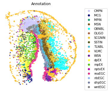
st.pl.space(adata,
            color=['Annotation'],
            pointsize=0.2,
            color_key=adata.uns['color_key'],
            show_legend='upper left',
            figsize=(5, 5))

Selection of genes of interest.

For example, we can choose highly spatially autocorrelated genes, or the genes that we are interested in. These potentially reflect signaling patterns that are uniform across spatial domains and have potentially interesting relationships cell-cell interaction events.

# Output directory:
save_dir = './model_result'
if not os.path.exists(save_dir):
    os.makedirs(save_dir)

Here, we use the st.tl.moran_i() to detect the genes that have spatial pattern.

m_degs = st.tl.moran_i(adata)
m_filter = m_degs[(m_degs.moran_i > 0.1) & (
    m_degs.moran_q_val < 0.05)].sort_values(by=['moran_i'], ascending=False)
m_filter.to_csv(os.path.join(save_dir, 'morani.csv'))

Then, filter down to genes morani >= 0.4 and expressed in at least 5% of cells (you can use different filtering criteria based on your own data).

m_filter = pd.read_csv(os.path.join(save_dir, 'morani.csv'))
m_filter

	Axolotl_ID	moran_i	moran_p_val	moran_z	moran_q_val
0	AMEX60DD017849	0.736978	0.005	76.417194	0.035229
1	AMEX60DD026264	0.734064	0.005	73.305991	0.035229
2	AMEX60DD026267	0.733105	0.005	74.481051	0.035229
3	AMEX60DD008655	0.718435	0.005	126.607623	0.035229
4	AMEX60DD021527	0.708344	0.005	75.485787	0.035229
...	...	...	...	...	...
1095	AMEX60DD008020	0.100284	0.005	9.845672	0.035229
1096	AMEX60DD028410	0.100264	0.005	9.701793	0.035229
1097	AMEX60DD025629	0.100262	0.005	10.519450	0.035229
1098	AMEX60DD011291	0.100216	0.005	9.744055	0.035229
1099	AMEX60DD028995	0.100118	0.005	9.751720	0.035229

1100 rows × 5 columns

m_filter = m_filter[m_filter['moran_i'] > 0.4]
n_cells = adata.n_obs
to_keep = []
for gene in m_filter.index:
    adata_sub = adata[:, gene]
    if scipy.sparse.issparse(adata_sub.X):
        n_cells_by_counts = adata_sub.X.getnnz(axis=0)
    else:
        n_cells_by_counts = np.count_nonzero(adata_sub.X, axis=0)
    if n_cells_by_counts >= 0.05 * n_cells:
        to_keep.append(gene)

targets = m_filter.loc[to_keep]

(optional) Specific processing of axolotl data, Homologous gene to human.

# Process to human-equivalent gene names(SOD2 maps to two different genes...)
adata = adata[:, adata.var['hs_gene'] != 'SOD2']
adata = adata[:, adata.var['hs_gene'] != "-"]
adata.var_names = adata.var['hs_gene']
targets = adata.var[adata.var['Axolotl_ID'].isin(
    targets['Axolotl_ID'])].index.tolist()
# here we add gene 'FZD2' to target gene list
targets = targets + ['FZD2']
targets

['ATF3',
 'VIM',
 'HBQ1',
 'RTN1',
 'HBG2',
 'GLUL',
 'NEUROD6',
 'PLP1',
 'SYNPR',
 'SST',
 'SCGN',
 'CPE',
 'NPTXR',
 'CXCL14',
 'FKBP1B',
 'FZD2']

Niche model

Niche model is used to predict the value of gene expression based on connections between categories within spatial neighborhoods.

Here, we use the target gene above to test our niche model. and assuming that the target gene expression follows a Poisson’s distribution(negative binomial and zero-inflated negative binomial are also provided in our function). Note that the Poisson’s distribution generally requires the UMI counts.

Process for Poisson regression

adata.layers['processed_counts'] = adata.X
adata.X = adata.layers['counts']

First, we fit the niche model, return coefficients (some other quantities of interest save to the AnnData object), and reg_lambda: discrete values of lambda regularization parameter to test n_jobs: number of parallel processes to run (genes to fit on in parallel).

niche_interp = st.tl.Niche_Model(
    adata,
    group_key='Annotation',
    genes=targets,
    smooth=False,
    normalize=False,
    log_transform=False,
    weights_mode="knn",
    distr="poisson",
    data_id="axolotl",
)

|-----> Note: argument provided to 'genes' represents the dependent variables for non-ligand-based analysis, but are used as independent variables for ligand-based analysis.
|-----> Preparing data: converting categories to one-hot labels for all samples.
|-----> Checking for pre-computed adjacency matrix for dataset axolotl...
|-----> Adjacency matrix loaded from file.

niche_coeffs, _ = niche_interp.GLMCV_fit_predict(
    reg_lambda=np.logspace(np.log(1e-3), np.log(1e-4), 3, base=np.exp(1)),
    n_jobs=1
)

niche_coeffs.to_csv(os.path.join(save_dir, 'niche_coeffs.csv'))
niche_df = pd.read_csv(os.path.join(save_dir, 'niche_coeffs.csv'), index_col=0)

Finally, we show the results of the niche model. First compute parameter significance.

niche_interp.get_effect_sizes(
    niche_df,
    significance_threshold=0.005,
)

|-----> With Poisson distribution assumed for dependent variable, using log-transformed data to compute sender-receiver effects...log key not found in adata, manually computing.
|-----> With a poisson assumption, it is recommended to fit to raw counts. Computing normalizations and transforms if applicable, but storing the results for later and fitting to the raw counts.
|-----> Log-transforming expression and storing in adata.layers['X_log1p'], adata.layers['X_norm_log1p'], adata.layers['X_M_s_log1p'], or adata.layers['X_norm_M_s_log1p'], depending on the normalizations and transforms that were specified.
|-----> With Poisson distribution assumed for dependent variable, using log-transformed data to compute sender-receiver effects...log key found in adata under key X_log1p.

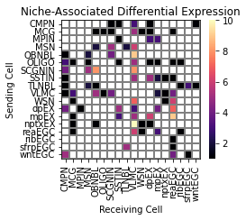
Niche model result 1:

type coupling analysis ignoring the effect of cell type in proximity to other cells of the same type (only hetero-cell type pairs).

niche_interp.type_coupling(
    cmap="magma",
    figsize=(4.4, 3.5),
    save_show_or_return='return')

Niche model result 2:

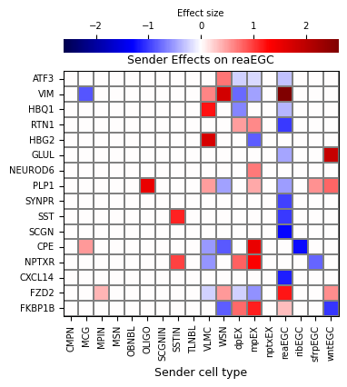
Sender effect: selecting reaEGC as the sender cell and visualizing effects on target genes in receiver cell types (all of the other cell types in the system). Visualization will plot the effect size, but qvals can be visualized using plot_mode'="qvals".

niche_interp.sender_effect_on_all_receivers(
    sender='reaEGC',
    figsize=(4.4, 5),
    save_show_or_return='return',
)

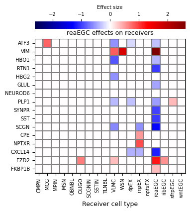
Niche model result 3:

Receiver effect: selecting reaEGC as the receiver cell, visualizing effects on target genes in reaEGC with all other cell types in the system as the sender. Visualization will plot the effect size, but qvals can be visualized using 'plot_mode'="qvals".

niche_interp.all_senders_effect_on_receiver(
    receiver='reaEGC',
    figsize=(4.4, 5),
    save_show_or_return="return",
)

Niche lr model

to predict a model for spatially-aware regression using the prevalence of and connections between categories within spatial neighborhoods and the cell type-specific expression of ligands and receptors to predict the regression target.

we choose the ligand-receptor pairs results based on the ./3.cci/1_cell-cell_communication_inference.ipynb. (In our case, we use ligand “L1CAM”, “PTN”, “TNC”,and receptor “ERBB3”, “SDC1”, and target genes above.)

First, we fit the Niche lr model, it is worth noting that cci_dir is the name of the directory containing human_mouse_signaling_network.csv. (Here, we provide species are human,mouse,axolotl to do below analysis). Other parameters are similar to st.tl.Niche_Model.

niche_lr_interp = st.tl.Niche_LR_Model(
    adata=adata,
    group_key='Annotation',
    genes=adata.var_names,
    smooth=False,
    normalize=False,
    log_transform=False,
    weights_mode="knn",
    niche_lr_r_lag=False,
    lig=["L1CAM", "PTN", "TNC"],
    rec=["ERBB3", "SDC1"],
    species="axolotl",
    data_id="axolotl",
    distr="poisson",
    cci_dir="/DATA/User/zuolulu/test/spateo-release/spateo/tools/database"
)

|-----> Note: argument provided to 'genes' represents the dependent variables for non-ligand-based analysis, but are used as independent variables for ligand-based analysis.
|-----> Predictor arrays for :class `Niche_LR_Model` are extremely sparse. It is recommended to provide categories to subset for :func `GLMCV_fit_predict`.
|-----> Preparing data: converting categories to one-hot labels for all samples.
|-----> Checking for pre-computed adjacency matrix for dataset axolotl...
|-----> Adjacency matrix loaded from file.
|-----> Preparing data: converting categories to one-hot labels for all samples.
|-----? Length of the provided list of ligands (input to 'l') does not match the length of the provided list of receptors (input to 'r'). This is fine, so long as all ligands and all receptors have at least one match in the other list.
Setting up Niche-L:R model using the following ligand-receptor pairs: [('L1CAM', 'ERBB3'), ('PTN', 'SDC1'), ('TNC', 'SDC1')]
|-----> Starting from 3 ligands and 2 receptors, found 3 ligand-receptor pairs.
|-----? Regression model has many predictors- consider measuring fewer ligands and receptors.
|-----> List of receptor-downstream genes was not provided- found these genes from the provided receptors: NRAS, CALM2, ITGB3, CAV1, PIK3R2, MAPK1, WNT1, CALML4, CALML3, CALML5, SHC1, SHC3, ITGAV, CAV2, SHC4, HSP90AA1, JAK1, HIF1A, CALM1, CALML6, PIK3CD, PIK3CB, MAPK3, SHC2, CAV3, GAB1, PLCG1, HSP90AB1, NOS3, CTNNB1, HRAS, HSP90B1, PIK3R1, KRAS, CALM3, JAK2, PIK3CA, PIK3R3, MYC, IRS1, PLCG2

nlr_coeffs, _ = niche_lr_interp.GLMCV_fit_predict(
    cat_key='Annotation',
    categories=['reaEGC', 'WSN'],
    reg_lambda=np.logspace(np.log(1e-3), np.log(1e-5), 3, base=np.exp(1)),
    n_jobs=1,
)

|-----> Optimal lambda regularization value for HSP90B1: 0.0010000000000000007.
|-----> Optimal lambda regularization value for KRAS: 0.0010000000000000007.
|-----> Optimal lambda regularization value for CTNNB1: 0.0010000000000000007.
|-----> Optimal lambda regularization value for HIF1A: 0.0010000000000000007.
|-----> Optimal lambda regularization value for PIK3R3: 0.0010000000000000007.
|-----> Optimal lambda regularization value for PLCG2: 1.0000000000000004e-05.
|-----> Optimal lambda regularization value for CAV1: 0.0010000000000000007.
|-----> Optimal lambda regularization value for CAV2: 0.0010000000000000007.
|-----> Optimal lambda regularization value for SHC2: 1.0000000000000004e-05.
|-----> Optimal lambda regularization value for NRAS: 0.0010000000000000007.
|-----> Optimal lambda regularization value for PIK3CA: 1.0000000000000004e-05.
|-----> Optimal lambda regularization value for SHC3: 0.0010000000000000007.
|-----> Optimal lambda regularization value for PIK3R1: 0.0010000000000000007.
|-----> Optimal lambda regularization value for CALML5: 0.0010000000000000007.
|-----> Optimal lambda regularization value for CALM3: 0.0010000000000000007.
|-----> Optimal lambda regularization value for CALM1: 0.0010000000000000007.
|-----> Optimal lambda regularization value for HRAS: 0.0010000000000000007.
|-----> Optimal lambda regularization value for SHC4: 0.0010000000000000007.
|-----> Optimal lambda regularization value for CALML4: 1.0000000000000004e-05.
|-----> Optimal lambda regularization value for PIK3CB: 0.0010000000000000007.
|-----> Optimal lambda regularization value for CALM2: 1.0000000000000004e-05.
|-----> Optimal lambda regularization value for GAB1: 1.0000000000000004e-05.
|-----> Optimal lambda regularization value for PLCG1: 0.0010000000000000007.
|-----> Optimal lambda regularization value for ITGB3: 9.999999999999996e-05.
|-----> Optimal lambda regularization value for CALML3: 0.0010000000000000007.
|-----> Optimal lambda regularization value for ITGAV: 0.0010000000000000007.
|-----> Optimal lambda regularization value for MAPK3: 0.0010000000000000007.

nlr_coeffs.to_csv(os.path.join(save_dir, 'nlr_coeffs.csv'))
nlr_df = pd.read_csv(os.path.join(save_dir, 'nlr_coeffs.csv'), index_col=0)

Finally, we show the results of the niche lr model.

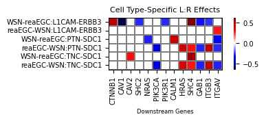
Niche lr model result 1:

Heatmap for coefficients:

We can choose specific sender-receiver pairs for the plot (recommended, otherwise plot will probably be large to the point of being uninterpretable), zero_center_cmap sets the colormap’s median color intensity to 0. Coefficients absolute value larger or smaller than mask_threshold are not assigned color in plot.

subset_cols = ["reaEGC-WSN", "WSN-reaEGC"]

niche_lr_interp.visualize_params(
    nlr_df,
    subset_cols=subset_cols if subset_cols is not None else None,
    cmap='seismic',
    zero_center_cmap=True,
    transpose=True,
    title="Cell Type-Specific L:R Effects",
    mask_threshold=0.25,
    xlabel="Downstream Genes",
    figsize=(5, 1),
    save_show_or_return='return',
)

0.5078398069446302