Note
This page was generated from
4_interactive_lasso_of_regions_of_interest.ipynb.
Interactive online version:
![]() .
Some tutorial content may look better in light mode.
.
Some tutorial content may look better in light mode.
Interactive lasso of regions of interest#
This notebook shows the how to lasso the reigion of interest(ROI), which stored as an anndata object after lasso to facilitate subsequent analysis.
[ ]:
To operate in jupyter or jupyterlab, you need to install the following plug-in.
[ ]:
conda install nodejs
jupyter labextension install @ jupyter-widgets/jupyterlab-manager
jupyter labextension install plotlywidget
jupyter labextension install @ jupyterlab/plotly-extension
[ ]:
import spateo as st
Load data#
We will be using a axolotl dataset from [Wei et al., 2022] (https://doi.org/10.1126/science.abp9444).
Here, we can get data directly from the functionst.sample.axolotl or link:
axolotl_2DPI: https://www.dropbox.com/s/7w2jxf41xazrqxo/axolotl_2DPI.h5ad?dl=1
[2]:
adata = st.sample_data.axolotl(filename='axolotl_2DPI.h5ad')
adata
[2]:
AnnData object with n_obs × n_vars = 7668 × 27324
    obs: 'CellID', 'spatial_leiden_e30_s8', 'Batch', 'cell_id', 'seurat_clusters', 'inj_uninj', 'D_V', 'inj_M_L', 'Annotation'
    var: 'Axolotl_ID', 'hs_gene'
    uns: 'Annotation_colors', '__type', 'color_key'
    obsm: 'X_spatial', 'spatial'
    layers: 'counts', 'log1p'
    obsp: 'connectivities', 'distances', 'spatial_connectivities', 'spatial_distances'
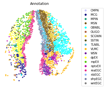
[3]:
st.pl.space(adata,
            color=['Annotation'],
            pointsize=0.2,
            color_key=adata.uns['color_key'],
            show_legend='upper left',
            figsize=(5, 5))
Lasso data#
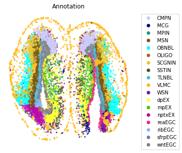
[4]:
a_lasso = st.tl.Lasso(adata)
[5]:
a_lasso.vi_plot(group='Annotation', group_color='Annotation_colors')
[10]:
sub_data = a_lasso.sub_adata
sub_data
[10]:
View of AnnData object with n_obs × n_vars = 1643 × 27324
    obs: 'CellID', 'spatial_leiden_e30_s8', 'Batch', 'cell_id', 'seurat_clusters', 'inj_uninj', 'D_V', 'inj_M_L', 'Annotation'
    var: 'Axolotl_ID', 'hs_gene'
    uns: 'Annotation_colors', '__type', 'color_key'
    obsm: 'X_spatial', 'spatial'
    layers: 'counts', 'log1p'
    obsp: 'connectivities', 'distances', 'spatial_connectivities', 'spatial_distances'
[11]:
st.pl.space(sub_data,
            color=['Annotation'],
            pointsize=0.2,
            color_key=adata.uns['color_key'],
            show_legend='upper left',
            figsize=(5, 5))