Note

This page was generated from 1_bin_scc.ipynb. Interactive online version: . Some tutorial content may look better in light mode.

1.Spatially constrained clustering (SCC) with binnning data

This notebook demonstrates how to perform basic clustering on a raw anndata object (spatial transcriptomic data) using spateo and SCC clustering.

Binning anndata object can be obtained with spateo.io functions from multiple spatial transcriptomic assays. (See the docs for spateo.io)

Packages

import spateo as st
import dynamo as dyn

2022-11-10 16:16:31.587596: I tensorflow/core/util/util.cc:169] oneDNN custom operations are on. You may see slightly different numerical results due to floating-point round-off errors from different computation orders. To turn them off, set the environment variable `TF_ENABLE_ONEDNN_OPTS=0`.
network.py (36): The next major release of pysal/spaghetti (2.0.0) will drop support for all ``libpysal.cg`` geometries. This change is a first step in refactoring ``spaghetti`` that is expected to result in dramatically reduced runtimes for network instantiation and operations. Users currently requiring network and point pattern input as ``libpysal.cg`` geometries should prepare for this simply by converting to ``shapely`` geometries.

|-----> setting visualization default mode in dynamo. Your customized matplotlib settings might be overritten.

Data source

bin60_h5ad: https://www.dropbox.com/s/c5tu4drxda01m0u/mousebrain_bin60.h5ad?dl=0

# Load binning data
fname_bin60 = "mousebrain_bin60.h5ad"
adata_bin60 = st.sample_data.mousebrain(fname_bin60)
adata_bin60

AnnData object with n_obs × n_vars = 7765 × 25691
    obs: 'area', 'n_counts'
    uns: '__type', 'pp', 'spatial'
    obsm: 'X_spatial', 'bbox', 'contour', 'spatial'
    layers: 'count', 'spliced', 'unspliced'

Normalization & Dimensional reduction

# Preprocessing
st.pp.filter.filter_genes(adata_bin60, min_cells=3, inplace=True)

# Normalization
dyn.pp.normalize_cell_expr_by_size_factors(adata_bin60, layers="X")

# Linear reduction
st.tl.pca_spateo(adata_bin60, n_pca_components=30)

# Identify neighbors(KNN)
dyn.tl.neighbors(adata_bin60, n_neighbors=30)

|-----> rounding expression data of layer: X during size factor calculation
|-----> size factor normalize following layers: ['X']
|-----> applying <ufunc 'log1p'> to layer<X>
|-----> set adata <X> to normalized data.
|-----> <insert> pp.norm_method to uns in AnnData Object.
|-----> Runing PCA on adata.X...
|-----> Start computing neighbor graph...
|-----------> X_data is None, fetching or recomputing...
|-----> fetching X data from layer:None, basis:pca
|-----> method arg is None, choosing methods automatically...
|-----------> method ball_tree selected
|-----> <insert> connectivities to obsp in AnnData Object.
|-----> <insert> distances to obsp in AnnData Object.
|-----> <insert> neighbors to uns in AnnData Object.
|-----> <insert> neighbors.indices to uns in AnnData Object.
|-----> <insert> neighbors.params to uns in AnnData Object.

AnnData object with n_obs × n_vars = 7765 × 21667
    obs: 'area', 'n_counts', 'Size_Factor', 'initial_cell_size'
    var: 'pass_basic_filter'
    uns: '__type', 'pp', 'spatial', 'neighbors'
    obsm: 'X_spatial', 'bbox', 'contour', 'spatial', 'X_pca'
    layers: 'count', 'spliced', 'unspliced'
    obsp: 'distances', 'connectivities'

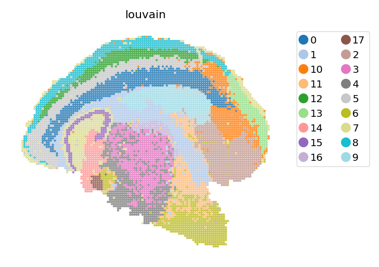
Vanilla louvain clustering

#louvain clustering
dyn.tl.louvain(adata_bin60, resolution=0.45)
st.pl.space(adata_bin60, color=['louvain'], show_legend="upper left", figsize=(4, 3), color_key_cmap="tab20")

|-----> accessing adj_matrix_key=distances built from args for clustering...
|-----> Detecting communities on graph...
|-----------> Converting graph_sparse_matrix to networkx object
|-----> [Community clustering with louvain] in progress: 100.0000%
|-----> [Community clustering with louvain] finished [28.6789s]

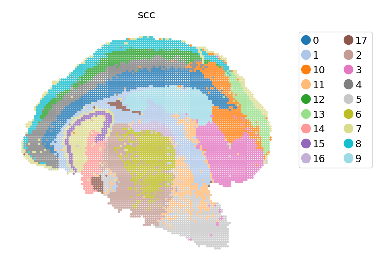
Spatially constrained clustering (SCC)

The SCC clustering function is implemented based on basic clustering methods (e.g. louvain, leiden, …), by replacing the input K-nearest neighbor(KNN) network, with the fusion of KNN and spatial neighbor network.

We adjust the computational weight of spatial nearness by adjusting the s_neigh argument. Typically, we set s_neigh according to the spatial arrangement of spots (i.e. the assay we use). For example, s_neigh could be 4, 8, 12, etc, in a squared array sequencing platform (such as Stereo-seq, …), and could be 6, 18, etc, in a hexagon platform (such as Visium, …). Larger s_neigh brings larger weight for spatial information, while we do not recommend setting s_neigh too big.

#scc clustering
st.tl.scc(
    adata_bin60,
    s_neigh=8,
    e_neigh=30,
    resolution=0.4,
    cluster_method="louvain",
    key_added="scc",
    pca_key="X_pca",
)
st.pl.space(adata_bin60, color=['scc'], show_legend="upper left", figsize=(4, 3), color_key_cmap="tab20")

|-----> Start computing neighbor graph...
|-----> method arg is None, choosing methods automatically...
|-----------> method ball_tree selected
|-----> <insert> connectivities to obsp in AnnData Object.
|-----> <insert> distances to obsp in AnnData Object.
|-----> <insert> neighbors to uns in AnnData Object.
|-----> <insert> neighbors.indices to uns in AnnData Object.
|-----> <insert> neighbors.params to uns in AnnData Object.
|-----> Start computing neighbor graph...
|-----> method arg is None, choosing methods automatically...
|-----------> method kd_tree selected
|-----> <insert> spatial_connectivities to obsp in AnnData Object.
|-----> <insert> spatial_distances to obsp in AnnData Object.
|-----> <insert> spatial_neighbors to uns in AnnData Object.
|-----> <insert> spatial_neighbors.indices to uns in AnnData Object.
|-----> <insert> spatial_neighbors.params to uns in AnnData Object.
|-----> using adj_matrix from arg for clustering...
|-----> Detecting communities on graph...
|-----------> Converting graph_sparse_matrix to networkx object
|-----> [Community clustering with louvain] in progress: 100.0000%
|-----> [Community clustering with louvain] finished [25.0800s]

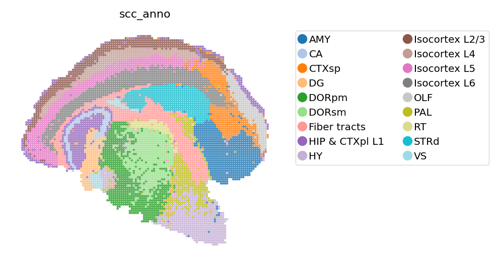
SCC clusters annotation

domain_annotations = [
    "Isocortex L6",
    "Fiber tracts",
    "CTXsp",
    "PAL",
    "Isocortex L4",
    "OLF",
    "DG",
    "CA",
    "RT",
    "VS",
    "DORpm",
    "AMY",
    "Isocortex L5",
    "HY",
    "DORsm",
    "HIP & CTXpl L1",
    "Isocortex L2/3",
    "STRd",
]

adata_bin60.obs['scc_anno'] = adata_bin60.obs['scc'].copy()
adata_bin60.rename_categories('scc_anno', domain_annotations)

st.pl.space(
    adata_bin60,
    color=['scc_anno'],
    show_legend="upper left",
    figsize=(4, 3),
    color_key_cmap="tab20"
)

adata_bin60.write("mousebrain_bin60_clustered.h5ad", compression="gzip")