Note

This page was generated from Interpolations.ipynb. Interactive online version: . Some tutorial content may look better in light mode.

3D spatial transcriptomics Interpolation

This notebook demonstrates the process of continuous expression pattern learning in the 3D volume model. Spateo contains the following four interpolation methods:

1. The methods (Shepard, Gaussian and Linear) contained in the VTK;

2. A new Gaussian Process method;

3. The SparseVFC method contained in the Dynamo;

4. A new Deep Learning method.

import warnings
import numpy as np
import spateo as st
import dynamo as dyn
warnings.filterwarnings("ignore")

2023-07-26 17:47:26.236300: W tensorflow/compiler/tf2tensorrt/utils/py_utils.cc:38] TF-TRT Warning: Could not find TensorRT

Load the data

cpo = [(553, 1098, 277), (1.967, -6.90, -2.21), (0, 0, 1)]

adata = st.sample_data.drosophila(filename="E7-9h_cellbin.h5ad")
adata.uns["pp"] = {}
adata.uns["__type"] = "UMI"
dyn.pp.normalize(adata)
dyn.pp.log1p(adata)
adata

AnnData object with n_obs × n_vars = 25921 × 8136
    obs: 'area', 'slices', 'anno_cell_type', 'anno_tissue', 'anno_germ_layer', 'actual_stage', 'spliced_Size_Factor', 'initial_spliced_cell_size', 'counts_X_Size_Factor', 'initial_counts_X_cell_size', 'Size_Factor', 'initial_cell_size', 'unspliced_Size_Factor', 'initial_unspliced_cell_size'
    uns: 'pp', '__type'
    obsm: '3d_align_spatial'
    layers: 'counts_X', 'spliced', 'unspliced', 'X_spliced', 'X_counts_X', 'X_unspliced'

# Down-sampling
from dynamo.tools import sample
sampling = sample(arr=np.asarray(adata.obs_names), n=10000, method="random", X=adata.obsm["3d_align_spatial"])
adata = adata[sampling, :]

Reconstruct the voxel model corresponding to the 3D spatial transcriptomics data

See also 3D Reconstruction for more details on 3D reconstructed models.

# Reconstruct point cloud model
pc, plot_cmap = st.tdr.construct_pc(adata=adata.copy(), spatial_key="3d_align_spatial", groupby="anno_tissue")

# Reconstruct mesh model
mesh, _, _ = st.tdr.construct_surface(pc=pc, alpha=0.6, cs_method="marching_cube", cs_args={"mc_scale_factor": 1.0}, smooth=5000, scale_factor=1.)

# Reconstruct voxel model
voxel, _ = st.tdr.voxelize_mesh(mesh=mesh, voxel_pc=pc, smooth=50)
voxel

UnstructuredGrid	Information
N Cells	17237
N Points	18780
X Bounds	-2.588e+02, 2.593e+02
Y Bounds	-1.092e+02, 9.780e+01
Z Bounds	-9.657e+01, 8.376e+01
N Arrays	0

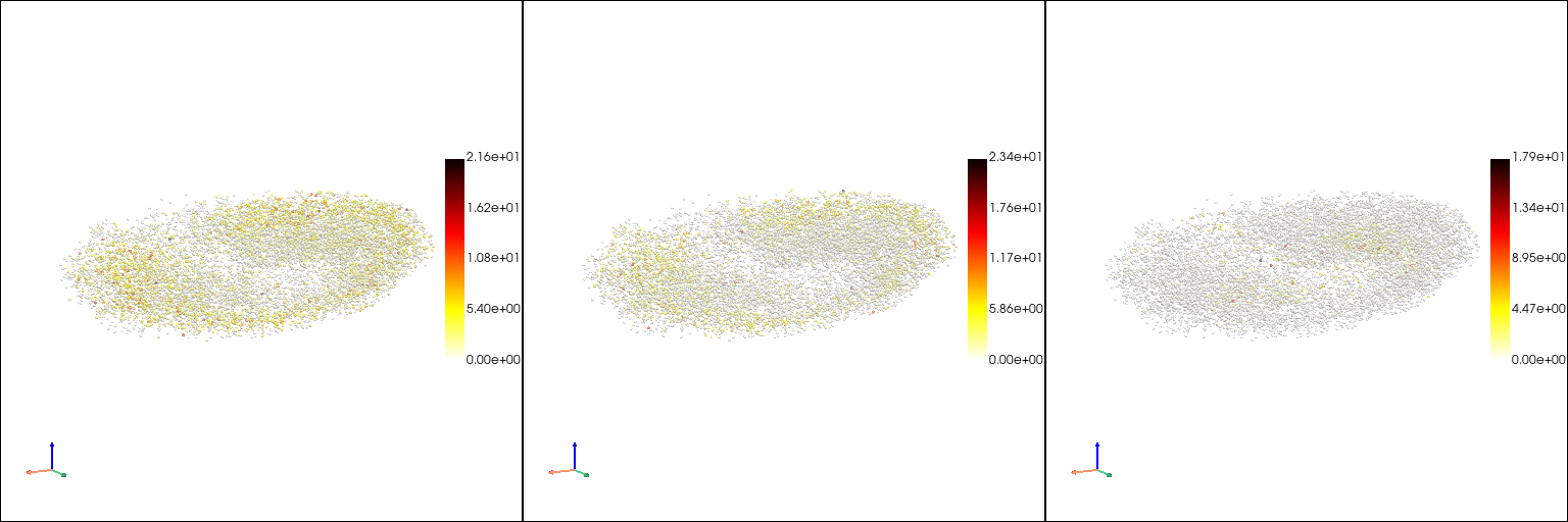
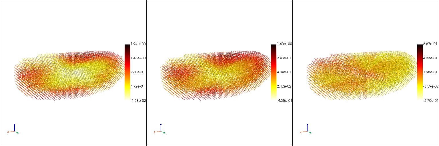
The raw gene expression patterns in the point cloud model

genes = ["Bacc", "HmgD", "Ance"]

# Add gene expression matrix to the point cloud model
pc_index=pc.point_data["obs_index"].tolist()
for gene_name in genes:
    exp = adata[pc_index, gene_name].X.flatten()
    st.tdr.add_model_labels(model=pc, labels=exp, key_added=gene_name, where="point_data",inplace=True)

st.pl.three_d_multi_plot(
    model=pc,
    key=genes,
    colormap="hot_r",
    opacity=0.5,
    model_style="points",
    jupyter="static",
    cpo=[cpo]
)

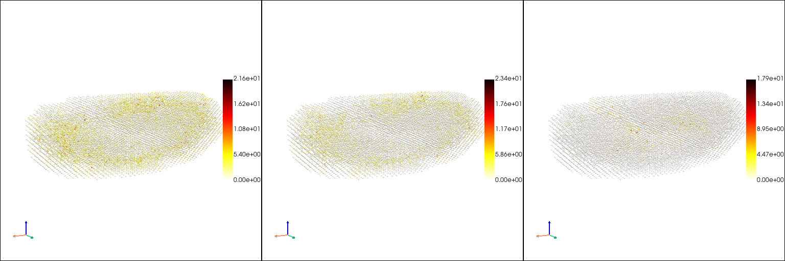
Learn a continuous mapping from space to gene expression pattern with the method contained in VTK

interpolated_vtk_adata = st.tdr.vtk_interpolation(source_adata=adata.copy(), spatial_key="3d_align_spatial", keys=genes, target_points=np.asarray(voxel.points), n_points=5)
interpolated_vtk_adata

|-----> Creating an adata object with the interpolated expression...
|-----> [VTKInterpolation] in progress: 100.0000%
|-----> [VTKInterpolation] finished [72.5322s]

AnnData object with n_obs × n_vars = 18780 × 3
    obsm: '3d_align_spatial'

interpolated_vtk_pc, _ = st.tdr.construct_pc(adata=interpolated_vtk_adata.copy(), spatial_key="3d_align_spatial", groupby=genes[0])
_pc_index=interpolated_vtk_pc.point_data["obs_index"].tolist()
for gene_name in genes[1:]:
    _exp = interpolated_vtk_adata[_pc_index, gene_name].X.flatten()
    st.tdr.add_model_labels(model=interpolated_vtk_pc, labels=_exp, key_added=gene_name, where="point_data",inplace=True)

st.pl.three_d_multi_plot(
    model=interpolated_vtk_pc,
    key=genes,
    colormap="hot_r",
    opacity=0.5,
    model_style="points",
    jupyter="static",
    cpo=[cpo]
)

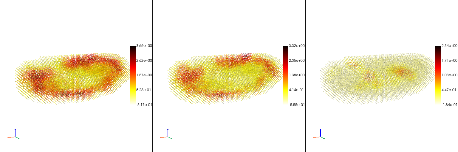
## Learn a continuous mapping from space to gene expression pattern with the Gaussian Process method

interpolated_gp_adata = st.tdr.gp_interpolation(source_adata=adata.copy(), spatial_key="3d_align_spatial", keys=genes, target_points=np.asarray(voxel.points), device="cpu")
interpolated_gp_adata

|-----> [Gaussian Process Regression] in progress: 100.0000%
|-----> [Gaussian Process Regression] finished [176.5625s]
|-----> Creating an adata object with the interpolated expression...
|-----> [GaussianProcessInterpolation] in progress: 100.0000%
|-----> [GaussianProcessInterpolation] finished [193.5424s]

AnnData object with n_obs × n_vars = 18780 × 3
    obsm: '3d_align_spatial'

interpolated_gp_pc, _ = st.tdr.construct_pc(adata=interpolated_gp_adata.copy(), spatial_key="3d_align_spatial", groupby=genes[0])
_pc_index=interpolated_gp_pc.point_data["obs_index"].tolist()
for gene_name in genes[1:]:
    _exp = interpolated_gp_adata[_pc_index, gene_name].X.flatten()
    st.tdr.add_model_labels(model=interpolated_gp_pc, labels=_exp, key_added=gene_name, where="point_data",inplace=True)

st.pl.three_d_multi_plot(
    model=interpolated_gp_pc,
    key=genes,
    colormap="hot_r",
    opacity=0.5,
    model_style="points",
    jupyter="static",
    cpo=[cpo]
)

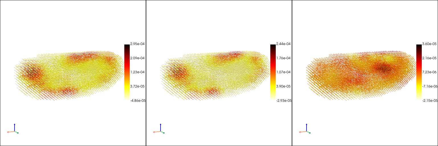
Learn a continuous mapping from space to gene expression pattern with sparseVFC method

interpolated_svfc_adata = st.tdr.kernel_interpolation(source_adata=adata.copy(), spatial_key="3d_align_spatial", keys=genes, target_points=np.asarray(voxel.points))
interpolated_svfc_adata

|-----> [SparseVFC] begins...
|-----> Sampling control points based on data velocity magnitude...
|-----> [SparseVFC] completed [0.3751s]
|-----> Creating an adata object with the interpolated expression...
|-----> [KernelInterpolation] in progress: 100.0000%
|-----> [KernelInterpolation] finished [0.9768s]

AnnData object with n_obs × n_vars = 18780 × 3
    obsm: '3d_align_spatial'

interpolated_svfc_pc, _ = st.tdr.construct_pc(adata=interpolated_svfc_adata.copy(), spatial_key="3d_align_spatial", groupby=genes[0])
_pc_index=interpolated_svfc_pc.point_data["obs_index"].tolist()
for gene_name in genes[1:]:
    _exp = interpolated_svfc_adata[_pc_index, gene_name].X.flatten()
    st.tdr.add_model_labels(model=interpolated_svfc_pc, labels=_exp, key_added=gene_name, where="point_data",inplace=True)

st.pl.three_d_multi_plot(
    model=interpolated_svfc_pc,
    key=genes,
    colormap="hot_r",
    opacity=0.5,
    model_style="points",
    jupyter="static",
    cpo=[cpo]
)

Learn a continuous mapping from space to gene expression pattern with deep learning method

interpolated_deep_adata = st.tdr.deep_intepretation(source_adata=adata.copy(), spatial_key="3d_align_spatial", keys=genes, target_points=np.asarray(voxel.points))
interpolated_deep_adata

Iter [     100] Time [9.8011] regression loss [8.0909] autoencoder loss [nan]
Model saved in path: model_buffer/
Iter [     200] Time [18.7046] regression loss [8.7426] autoencoder loss [nan]
Model saved in path: model_buffer/
Iter [     300] Time [27.0023] regression loss [8.3314] autoencoder loss [nan]
Model saved in path: model_buffer/
Iter [     400] Time [36.9290] regression loss [8.4856] autoencoder loss [nan]
Model saved in path: model_buffer/
Iter [     500] Time [45.0048] regression loss [8.3843] autoencoder loss [nan]
Model saved in path: model_buffer/
Iter [     600] Time [53.7922] regression loss [8.7756] autoencoder loss [nan]
Model saved in path: model_buffer/
Iter [     700] Time [63.0616] regression loss [9.2791] autoencoder loss [nan]
Model saved in path: model_buffer/
Iter [     800] Time [72.5802] regression loss [9.0534] autoencoder loss [nan]
Model saved in path: model_buffer/
Iter [     900] Time [82.7186] regression loss [8.4884] autoencoder loss [nan]
Model saved in path: model_buffer/
Iter [    1000] Time [92.2158] regression loss [8.9910] autoencoder loss [nan]
Model saved in path: model_buffer/
|-----> Creating an adata object with the interpolated expression...
|-----> [DeepLearnInterpolation] in progress: 100.0000%
|-----> [DeepLearnInterpolation] finished [92.9216s]

AnnData object with n_obs × n_vars = 18780 × 3
    obsm: '3d_align_spatial'

interpolated_deep_pc, _ = st.tdr.construct_pc(adata=interpolated_deep_adata.copy(), spatial_key="3d_align_spatial", groupby=genes[0])
_pc_index=interpolated_deep_pc.point_data["obs_index"].tolist()
for gene_name in genes[1:]:
    _exp = interpolated_deep_adata[_pc_index, gene_name].X.flatten()
    st.tdr.add_model_labels(model=interpolated_deep_pc, labels=_exp, key_added=gene_name, where="point_data",inplace=True)

st.pl.three_d_multi_plot(
    model=interpolated_deep_pc,
    key=genes,
    colormap="hot_r",
    opacity=0.5,
    model_style="points",
    jupyter="static",
    cpo=[cpo]
)

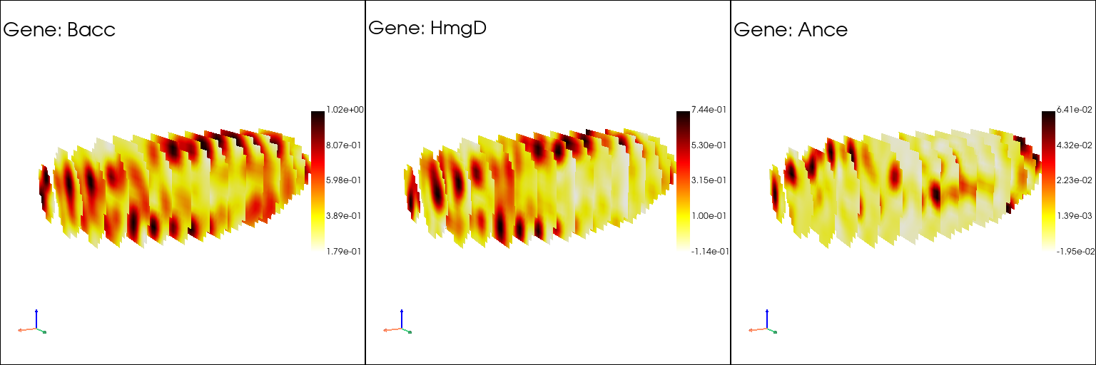
Slice the voxel model to observe the gene expression inside the model

for gene_name in genes:
    voxel.point_data[gene_name] = np.asarray(interpolated_gp_adata[:, gene_name].X)

voxel_slices_x = st.tdr.three_d_slice(model=voxel, method="axis", n_slices=15, axis="x")

st.pl.three_d_multi_plot(
    model=st.tdr.collect_models([voxel_slices_x]),
    key=genes,
    model_style="surface",
    colormap="hot_r",
    ambient=0.5,
    jupyter="static",
    cpo=[cpo],
    shape=(1, 3),
    text=[f"\nGene: {gene_name}\n" for gene_name in genes],
    text_kwargs={"text_size": 15, "text_font": "arial"},
)